Graph Algorithms
A Minecraft world is a graph. Every chunk you have visited is a vertex. Every path you have walked between chunks is an edge. When you decide how to get from your base to the village, you are running a graph algorithm in your head — you are picking which of three roughly equal moves to make. This page makes those moves explicit and gives them names.
The first graph algorithm published in a research journal came out of a Bell Labs paper by Edward Moore in 1959. He had built a maze-solver for Claude Shannon's mechanical mouse Theseus, which Shannon had wired up in 1950 to navigate a switchboard maze. Moore's algorithm for finding the shortest path through a maze is what we now call breadth-first search. Three years earlier, in 1956, Edsger Dijkstra was sitting in a coffee shop in Amsterdam with his fiancée and 20 minutes to kill. He wanted to demonstrate that the new ARMAC computer could do something that sounded impossible. He invented his shortest-path algorithm in his head, on the spot, and published it in 1959 as a one-page paper. Both algorithms still ship in every routing system on the planet — your GPS, your video-game pathfinder, the way your packets find a server.
You already have a graph to work with — the Graph class from ds-graphs, which stores vertices and their neighbors as an adjacency list. The shape: add_edge(u, v) records that u and v are connected, and neighbors(v) returns the list of vertices reachable from v in one hop. Every algorithm on this page works against that interface. Open algo_graph.py and rebuild the graph you used last lesson.
from graphs import Graph

world = Graph()
for u, v in [("base", "river"), ("base", "forest"), ("river", "village"),
             ("forest", "cave"), ("village", "mountain"), ("cave", "mountain")]:
    world.add_edge(u, v)
That is a small Minecraft map: your base connects to the river and the forest, the river leads to the village, the forest leads to the cave, and both the village and the cave reach the mountain.
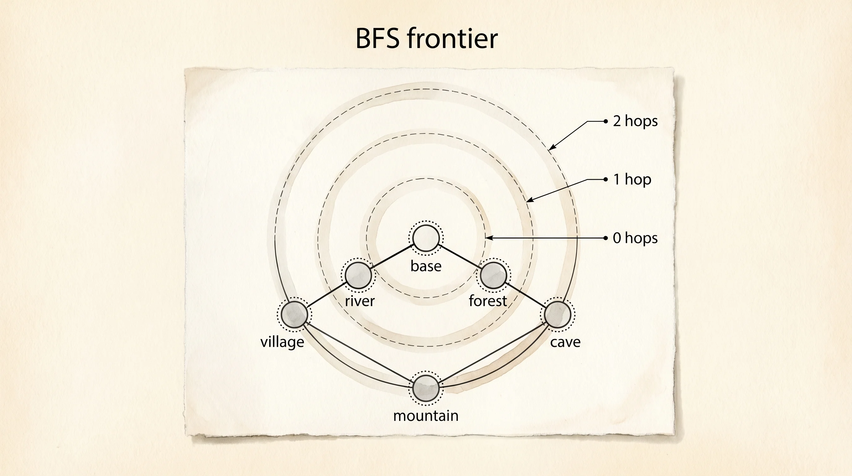
Breadth-first search walks the graph in rings. You stand at the start, write down every vertex one step away, then every vertex two steps away, then three. The trick is the queue — a first-in-first-out list. You push the start vertex onto the queue, then in a loop you pop the front vertex, mark it visited, and push every unvisited neighbor onto the back. Because the queue is FIFO, you always process the closer vertices before the farther ones.
from collections import deque

def bfs(graph, start, trace=False):
    visited = {start}
    queue = deque([start])
    order = []
    while queue:
        if trace:
            print(f"queue: {list(queue)}")
        current = queue.popleft()
        order.append(current)
        for neighbor in graph.neighbors(current):
            if neighbor not in visited:
                visited.add(neighbor)
                queue.append(neighbor)
    return order

bfs(world, "base", trace=True)
queue: ['base']
queue: ['river', 'forest']
queue: ['forest', 'village']
queue: ['village', 'cave']
queue: ['cave', 'mountain']
queue: ['mountain']Read the queue line by line. After the first pop, the base's two neighbors (river, forest) are sitting in the queue. After the second pop, river's neighbor (village) joins the back. After the third, forest's neighbor (cave) joins. The expansion is in rings — everything one step from base goes in before anything two steps from base does. BFS is the right algorithm whenever "fewest hops" is the question — friend-of-a-friend on social networks, the cheapest pawn move that captures a piece, the shortest road in a city where every road has the same length.
Depth-first search uses a stack instead of a queue. A stack is last-in-first-out. You push the start, pop the most recently added vertex, push its neighbors. Because the most recent neighbor goes in last and comes out first, DFS plunges down one path until it dead-ends, then backtracks to the most recent fork and tries another branch.
def dfs(graph, start, trace=False):
    visited = set()
    stack = [start]
    order = []
    while stack:
        if trace:
            print(f"stack: {stack}")
        current = stack.pop()
        if current in visited:
            continue
        visited.add(current)
        order.append(current)
        for neighbor in graph.neighbors(current):
            if neighbor not in visited:
                stack.append(neighbor)
    return order

dfs(world, "base", trace=True)
stack: ['base']
stack: ['river', 'forest']
stack: ['river', 'cave']
stack: ['river', 'mountain']
stack: ['river', 'village']
stack: ['river']Same graph, different walking style. After base is popped, the stack holds [river, forest]. The next pop takes forest (the most recent), which adds cave. Then cave is popped, which adds mountain. Then mountain is popped, which adds village. By the time the algorithm gets back to river, the entire branch through forest has already been walked. DFS is the right move when you are looking for any path through a maze, when you are checking if a graph has a cycle, or when the answer lives at the leaves of a tree and the tree is too wide to walk in rings.
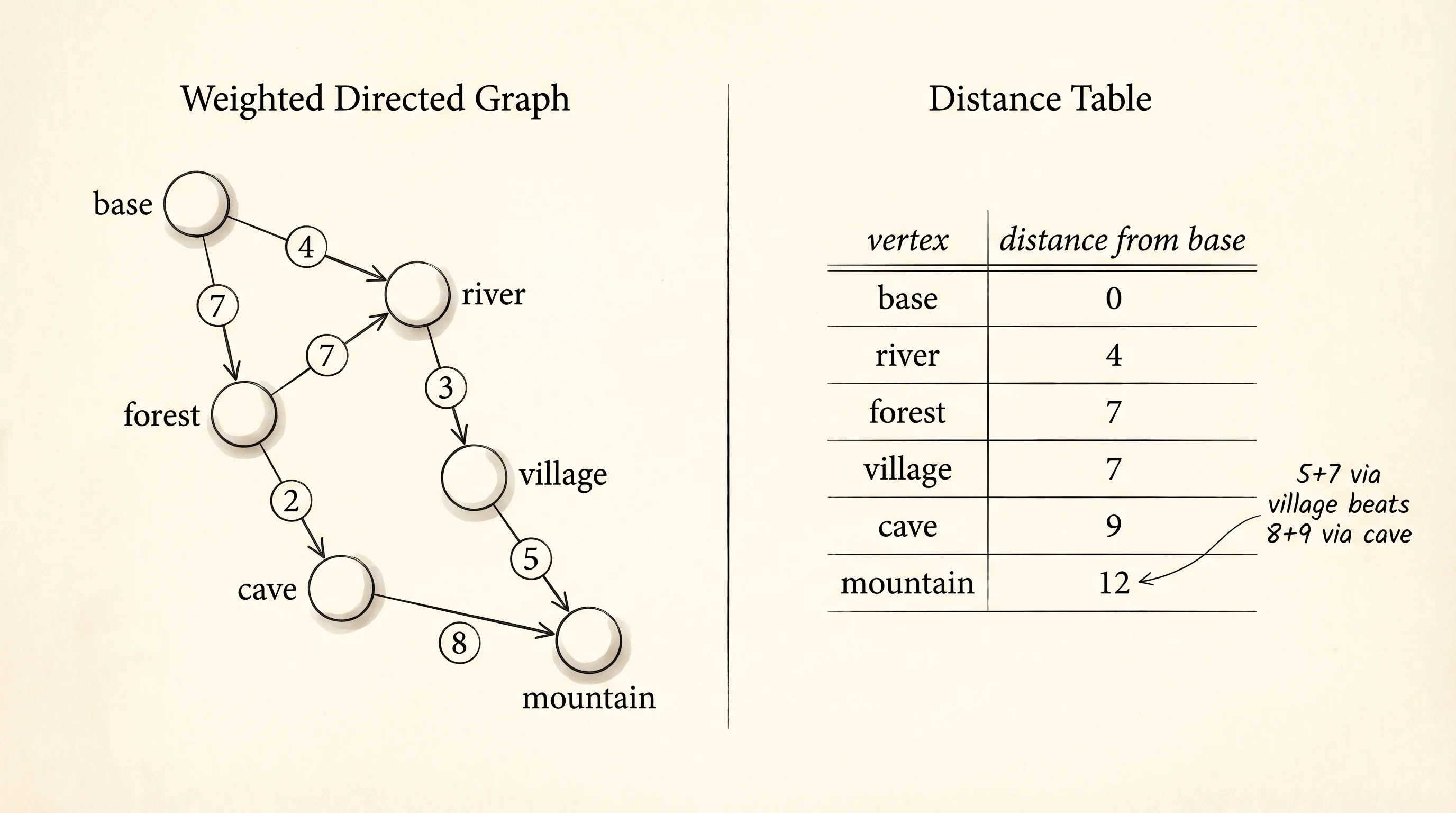
Dijkstra's algorithm is BFS with a backpack of fuel. Each edge now has a weight — the road from base to river takes 4 minutes; the road from base to forest takes 7. The cheapest route is no longer the one with the fewest hops, it is the one with the smallest total weight. Dijkstra solves it by keeping a distance table that holds the cheapest known cost from the start to every vertex, and a priority queue that always pops the cheapest unvisited vertex. The heapq module in Python is a min-heap, which is what you want.
The Graph class from ds-graphs stored unweighted edges. Wrap it in a small dict that maps (u, v) to its weight, or rebuild the graph as a dict keyed by vertex with a list of (neighbor, weight) tuples. The version below uses the second approach so the example stays one file.
import heapq

weighted = {
    "base": [("river", 4), ("forest", 7)],
    "river": [("base", 4), ("village", 3)],
    "forest": [("base", 7), ("cave", 2)],
    "village": [("river", 3), ("mountain", 5)],
    "cave": [("forest", 2), ("mountain", 8)],
    "mountain": [("village", 5), ("cave", 8)],
}

def dijkstra(graph, start, trace=False):
    distances = {v: float("inf") for v in graph}
    distances[start] = 0
    heap = [(0, start)]
    while heap:
        if trace:
            print(f"distances: {distances}")
        cost, current = heapq.heappop(heap)
        if cost > distances[current]:
            continue
        for neighbor, weight in graph[current]:
            new_cost = cost + weight
            if new_cost < distances[neighbor]:
                distances[neighbor] = new_cost
                heapq.heappush(heap, (new_cost, neighbor))
    return distances

dijkstra(weighted, "base", trace=True)
distances: {'base': 0, 'river': inf, 'forest': inf, 'village': inf, 'cave': inf, 'mountain': inf}
distances: {'base': 0, 'river': 4, 'forest': 7, 'village': inf, 'cave': inf, 'mountain': inf}
distances: {'base': 0, 'river': 4, 'forest': 7, 'village': 7, 'cave': inf, 'mountain': inf}
distances: {'base': 0, 'river': 4, 'forest': 7, 'village': 7, 'cave': 9, 'mountain': inf}
distances: {'base': 0, 'river': 4, 'forest': 7, 'village': 7, 'cave': 9, 'mountain': 12}
distances: {'base': 0, 'river': 4, 'forest': 7, 'village': 7, 'cave': 9, 'mountain': 12}Read the table top to bottom and watch the infinities collapse into real numbers. Round 1: base is 0, everything else is unreachable. Round 2: river and forest become 4 and 7 — the direct edges from base. Round 3: village becomes 7, the cost through river. Round 4: cave becomes 9, the cost through forest. Round 5: mountain becomes 12, the cost through village (which is cheaper than cave's 9 + 8 = 17). The final table tells you the shortest distance from base to every other vertex in the world.
Dijkstra has one rule it cannot break: every edge weight must be non-negative. If a road can have a negative time — say, a teleporter that gives you back 5 minutes — the algorithm produces wrong answers because it commits to a vertex's distance the moment it pops it from the heap. Bellman-Ford, the algorithm that handles negative edges, runs in O(VE) instead of O((V + E) log V) and you reach for it when you have to.
You can find your way through any map. Some problems are not maps, though — they are recursive trees that secretly repeat the same subtree over and over. The fix is to remember.