Searching

The dumbbell rack is sorted now, lightest on the left, heaviest on the right. You walk in, you need the 50. You can scan the whole rack from one end like a beginner, or you can use the order someone already paid for. The order is what makes the second method possible. Without it you are stuck doing the dumb thing.

Linear search is the dumb thing. You start at the left end and check each weight one at a time until you find the 50. If the rack has 30 dumbbells you check at most 30. If the gym has 300 you might check 300. The cost grows with the size of the rack — O(n), which you met last lesson. People knew this without naming it. The break came in 1946 at the Moore School in Philadelphia, where John Mauchly was teaching a summer lecture series on the new ENIAC. Mauchly described an idea for searching a sorted table by repeatedly cutting it in half. The first cleanly working version of the algorithm in code came in 1960 from Derrick Henry Lehmer at Berkeley, who fixed the off-by-one bugs that the early sketches kept making. Half the world's published binary searches have been buggy ever since — Jon Bentley wrote a famous 1986 column saying that of every binary search ever written by professionals, an alarming fraction did not work on the largest or smallest input.

Open searching.py and write linear search first. It is six lines.

def linear_search(nums, target):
    for i, value in enumerate(nums):
        if value == target:
            return i
    return -1
 
print(linear_search([10, 20, 30, 40, 50, 60, 70, 80], 50))

It prints 4 — index 4 holds 50. The function does not assume the list is sorted. That is the only good thing about it. Now write binary search, which does assume the list is sorted, and earns a much better cost in return. The shape: keep two pointers, lo and hi, marking the slice of the list you are still considering. Look at the middle. If the middle is the target, you are done. If the target is smaller, throw away the right half. If the target is bigger, throw away the left half. Repeat until lo passes hi.

def binary_search(nums, target, trace=False):
    lo = 0
    hi = len(nums) - 1
    while lo <= hi:
        mid = (lo + hi) // 2
        if trace:
            print(f"lo={lo}, hi={hi}, mid={mid}, nums[mid]={nums[mid]}")
        if nums[mid] == target:
            return mid
        if nums[mid] < target:
            lo = mid + 1
        else:
            hi = mid - 1
    return -1
 
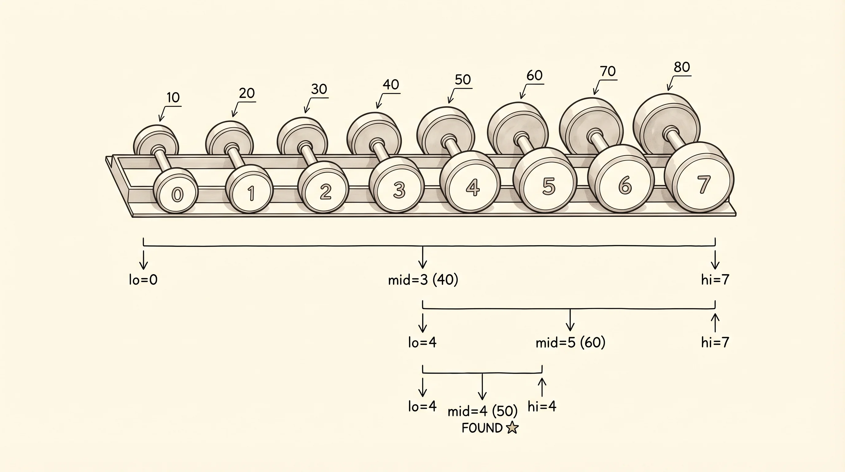
binary_search([10, 20, 30, 40, 50, 60, 70, 80], 50, trace=True)

Run it and read the trace.

lo=0, hi=7, mid=3, nums[mid]=40
lo=4, hi=7, mid=5, nums[mid]=60
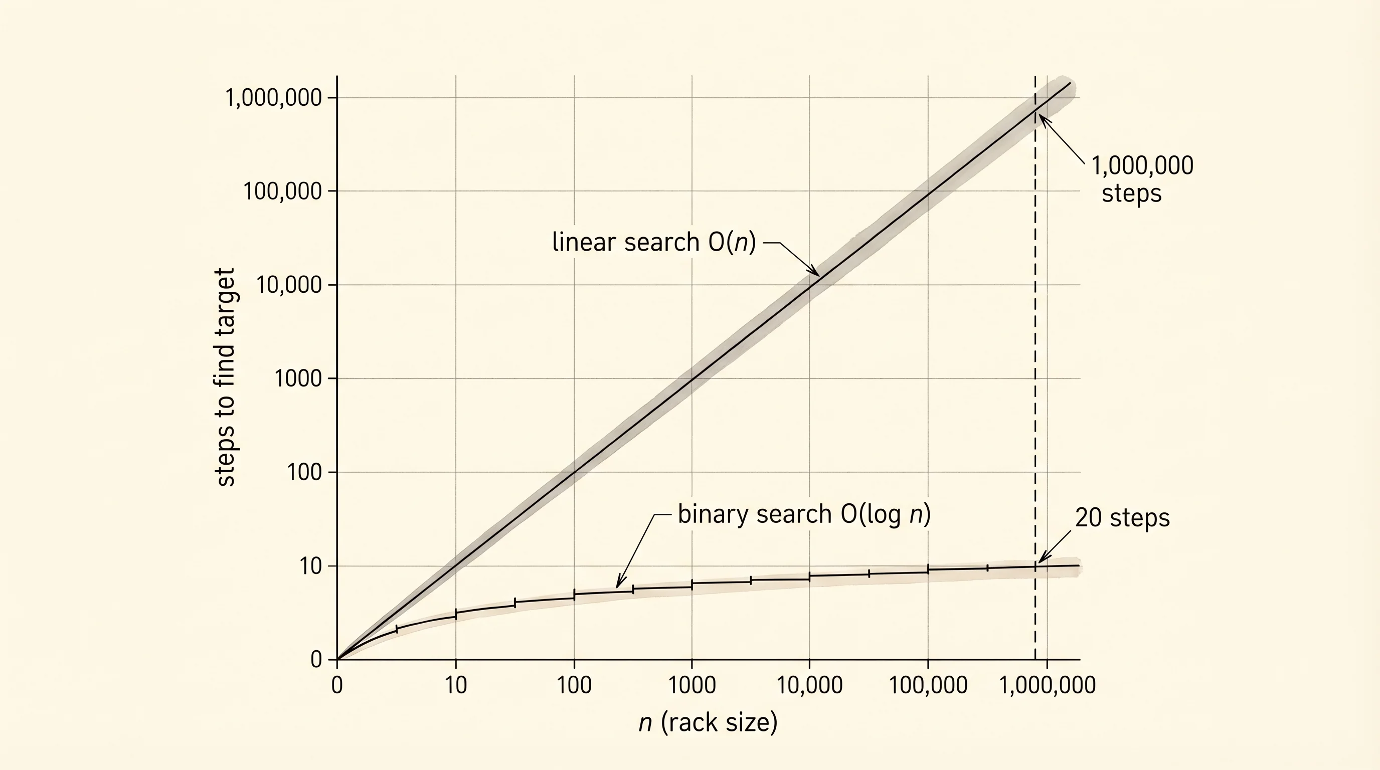
lo=4, hi=4, mid=4, nums[mid]=50

Three steps for a list of 8 elements. The first step covered the whole rack. The second covered the right half. The third covered a single slot, which happened to be the answer. That is the halving move. Each step throws out half of what is left. For a list of 1 million elements binary search takes at most 20 steps because 2^20 is about 1 million. Linear search on the same list takes up to 1 million steps. The trade is real but it has a price: the list has to be sorted first, and sorting costs O(n log n). You only earn binary search's payoff when you are going to search the same list many times.

Time them against each other. The timer decorator from big-o works here too — copy it in.

import time
from typing import Callable
 
def timer(fn: Callable) -> Callable:
    def wrapped(*args, **kwargs):
        start = time.perf_counter()
        result = fn(*args, **kwargs)
        elapsed = time.perf_counter() - start
        print(f"{fn.__name__} on n={len(args[0])} took {elapsed * 1000:.4f} ms")
        return result
    return wrapped
 
@timer
def linear(nums, target):
    return linear_search(nums, target)
 
@timer
def binary(nums, target):
    return binary_search(nums, target)
 
big = list(range(10_000_000))
linear(big, 9_999_999)
binary(big, 9_999_999)

linear on n=10000000 took 421.1820 ms
binary on n=10000000 took 0.0070 ms

Same answer, both correct. Linear walked nearly 10 million elements. Binary walked 24. The 421 ms is half a second your user spends staring at a frozen screen. The 0.007 ms is below human perception. That gap is why every database index in the world is built on a tree structure — they are searching billions of rows and the difference is an outage versus a successful query.

The off-by-one Bentley warned about lives in two spots. The first is the loop condition: while lo <= hi, not while lo < hi. If you write the strict version you skip the case where the target is the last remaining element. The second is the pointer updates: lo = mid + 1 and hi = mid - 1, not lo = mid and hi = mid. If you write the non-plus-one version your loop never narrows when the target is between two elements and the program loops forever. The standard library hides these traps inside bisect.bisect_left, which is the binary search you will reach for in real code. You wrote it once by hand so you understand what it costs to get it right.

A question. The trace above ran on a list where the target was present. What does the trace look like if the target is not in the list? Try it: binary_search([10, 20, 30, 40, 50, 60, 70, 80], 35, trace=True). The function prints three rows again — lo=0,hi=7,mid=3, lo=0,hi=2,mid=1, lo=2,hi=2,mid=2 — and then the loop condition fails because lo becomes 3 and hi is 2. It returns -1. The number of steps is the same; the answer is "not found." Binary search costs O(log n) whether or not the target exists.

You can find anything in a sorted list in 20 steps. Loops and pointers got you here. A function that calls itself can cut problems in half the same way, but with a different shape on the page.