Sorting

The dumbbell rack at the end of leg day looks like a crime scene. A 35 sits next to a 70 sits next to a 15. Re-racking is sorting. The job has a clean rule — put them in order, lightest to heaviest — and four different ways to actually do it. Each way is an algorithm, and each one trades work for cleverness in a different ratio.

The first sorting algorithm written down for a real machine was mergesort. John von Neumann sketched it in 1945 while working out what programs the EDVAC would need. Computers were still being assembled. Memory was made of mercury delay lines that held bits as sound waves. Von Neumann saw that the cleanest way to sort a long list was to split it into halves, sort each half, then merge the two sorted halves with one pass. Fifteen years later, in 1960, a 26-year-old Tony Hoare was at the National Physical Laboratory in London on a project to translate Russian into English. He needed to sort the words in a sentence to look them up in a dictionary. He invented quicksort on a beach holiday before he came back to work. Bubble sort and insertion sort are older and dumber and people still teach them first because they show the shape of the problem.

Start with bubble sort, the rack-walk method. You pass through the rack from left to right. Every time you see a heavier dumbbell to the left of a lighter one, you swap them. After one pass the heaviest dumbbell has bubbled all the way to the right end. After a second pass the second-heaviest has bubbled to its place. After n passes the rack is sorted. Open sorts.py.

def bubble_sort(nums, trace=False):
    arr = list(nums)
    n = len(arr)
    for pass_num in range(n - 1):
        swapped = False
        for i in range(n - 1 - pass_num):
            if arr[i] > arr[i + 1]:
                arr[i], arr[i + 1] = arr[i + 1], arr[i]
                swapped = True
        if trace:
            print(f"after pass {pass_num + 1}: {arr}")
        if not swapped:
            break
    return arr
 
bubble_sort([5, 1, 4, 2, 8, 3], trace=True)

Run it. The print after every pass shows the rack mid-sort.

after pass 1: [1, 4, 2, 5, 3, 8]
after pass 2: [1, 2, 4, 3, 5, 8]
after pass 3: [1, 2, 3, 4, 5, 8]

The 8 floats to the end on pass 1. The 5 settles on pass 2. By pass 3 the array is sorted, and on pass 4 the function notices nothing swapped and quits. The visible bubbling is where the name comes from. The cost is bad: in the worst case, where the array is reverse-sorted, bubble sort does about n²/2 comparisons. At n=10 that is 50. At n=10000 it is 50 million. Bubble sort is the algorithm you teach, not the one you ship.

Insertion sort is also O(n²) but it earns its keep. The idea is the way you sort a hand of playing cards as you pick them up: take each new card and slide it left until it sits in the right place against the cards already in your hand.

def insertion_sort(nums, trace=False):
    arr = list(nums)
    for i in range(1, len(arr)):
        current = arr[i]
        j = i - 1
        while j >= 0 and arr[j] > current:
            arr[j + 1] = arr[j]
            j -= 1
        arr[j + 1] = current
        if trace:
            print(f"after inserting index {i}: {arr}")
    return arr
 
insertion_sort([5, 1, 4, 2, 8, 3], trace=True)

after inserting index 1: [1, 5, 4, 2, 8, 3]
after inserting index 2: [1, 4, 5, 2, 8, 3]
after inserting index 3: [1, 2, 4, 5, 8, 3]
after inserting index 4: [1, 2, 4, 5, 8, 3]
after inserting index 5: [1, 2, 3, 4, 5, 8]

The left side of the array stays sorted from the moment the loop starts. Each new element finds its slot in the sorted prefix. On a nearly-sorted input, insertion sort runs in O(n) — every element is already close to home. That is why Python's real sort, Timsort, uses insertion sort for small sub-arrays.

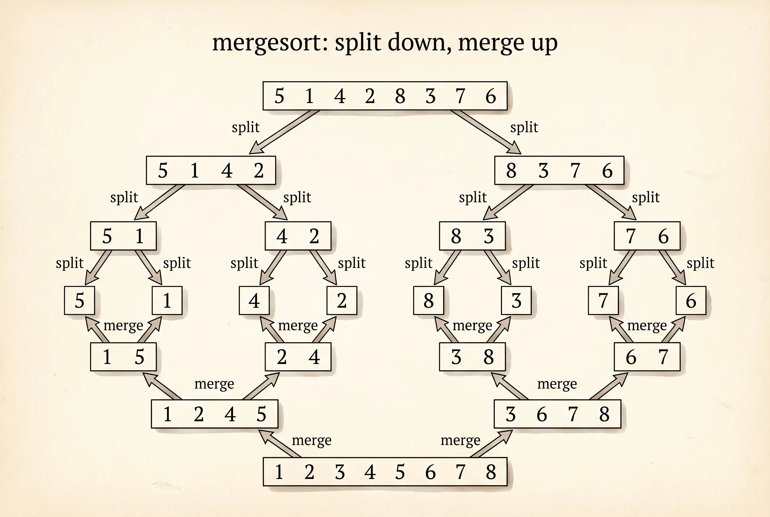
Mergesort is the von Neumann move. Split the rack in half. Sort each half by calling yourself on it. Then walk both halves with two fingers, taking whichever side is lighter, until both halves are merged into one sorted rack. Recursion will get its own lesson; for now, treat the function calling itself as the natural way to split a problem in two.

def merge_sort(nums, trace=False, depth=0):
    if len(nums) <= 1:
        return list(nums)
    mid = len(nums) // 2
    left = merge_sort(nums[:mid], trace, depth + 1)
    right = merge_sort(nums[mid:], trace, depth + 1)
    merged = merge(left, right)
    if trace:
        indent = "  " * depth
        print(f"{indent}merge {left} + {right} -> {merged}")
    return merged
 
def merge(left, right):
    result = []
    i = j = 0
    while i < len(left) and j < len(right):
        if left[i] <= right[j]:
            result.append(left[i])
            i += 1
        else:
            result.append(right[j])
            j += 1
    result.extend(left[i:])
    result.extend(right[j:])
    return result
 
merge_sort([5, 1, 4, 2, 8, 3], trace=True)

The trace shows each merge with its depth indented:

      merge [5] + [1] -> [1, 5]
        merge [2] + [8] -> [2, 8]
      merge [4] + [2, 8] -> [2, 4, 8]
    merge [1, 5] + [2, 4, 8] -> [1, 2, 4, 5, 8]
  merge [1, 2, 4, 5, 8] + [3] -> [1, 2, 3, 4, 5, 8]

Mergesort is O(n log n). The list splits log n times and each split costs n work to merge back. At n=1 million it does about 20 million operations instead of bubble sort's trillion. The cost is memory — mergesort allocates new lists at each level. That is the trade.

Quicksort is the same recursive shape with a sneakier partition step. Pick any element as a pivot. Walk the array once, putting everything smaller than the pivot on its left and everything bigger on its right. Recurse on both sides.

def quick_sort(nums, trace=False, depth=0):
    if len(nums) <= 1:
        return list(nums)
    pivot = nums[0]
    smaller = [x for x in nums[1:] if x <= pivot]
    bigger = [x for x in nums[1:] if x > pivot]
    if trace:
        indent = "  " * depth
        print(f"{indent}pivot={pivot}, smaller={smaller}, bigger={bigger}")
    return quick_sort(smaller, trace, depth + 1) + [pivot] + quick_sort(bigger, trace, depth + 1)
 
quick_sort([5, 1, 4, 2, 8, 3], trace=True)

pivot=5, smaller=[1, 4, 2, 3], bigger=[8]
  pivot=1, smaller=[], bigger=[4, 2, 3]
    pivot=4, smaller=[2, 3], bigger=[]
      pivot=2, smaller=[], bigger=[3]

Quicksort averages O(n log n) and beats mergesort in practice because it sorts in place (the textbook version, not this teaching one) and touches fewer cache lines. Its worst case is O(n²) when the pivot is always the smallest or largest element — pick a random pivot and that worst case becomes very unlikely.

Python ships with a sort. Calling sorted([5, 1, 4, 2, 8, 3]) runs Timsort, an algorithm Tim Peters wrote in 2002 specifically for Python. Timsort scans the input for already-sorted runs, uses insertion sort on small chunks, and merges the runs. On real-world data — which is rarely perfectly random — it often beats pure quicksort. You will reach for sorted() from now on. The four sorts above are the workout that earns the right to use it.

You can put the rack in order. The next move pays you back: a sorted rack lets you find any dumbbell without checking every slot.