Big O

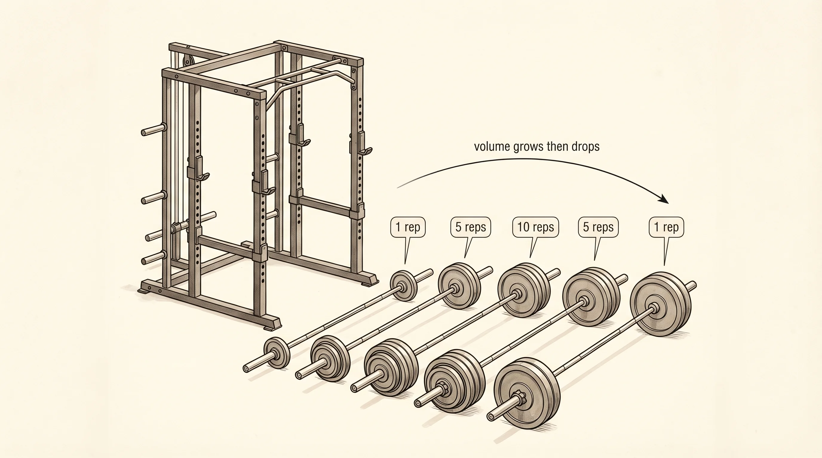
A workout earns its soreness from volume. One set of squats with the bar is nothing. Five sets is real work. A pyramid that ramps every set up to a heavy single and back down can leave you flat for two days. The number of reps grew, and the cost grew with it. Big O is the same idea applied to code: as the input gets bigger, how fast does the work pile up?

The notation came out of math, not programming. Paul Bachmann was a German number theorist who in 1894 wanted a compact way to say "this function grows roughly like that one, give or take a constant factor." He wrote a capital O followed by the dominant term and the rest of the math world started using it the same week. For 80 years it lived in pure math papers. In 1976 Donald Knuth, the Stanford professor writing his lifelong series The Art of Computer Programming, dragged the notation into programming and it never left. Today every algorithm gets two labels: what it does, and its Big O.

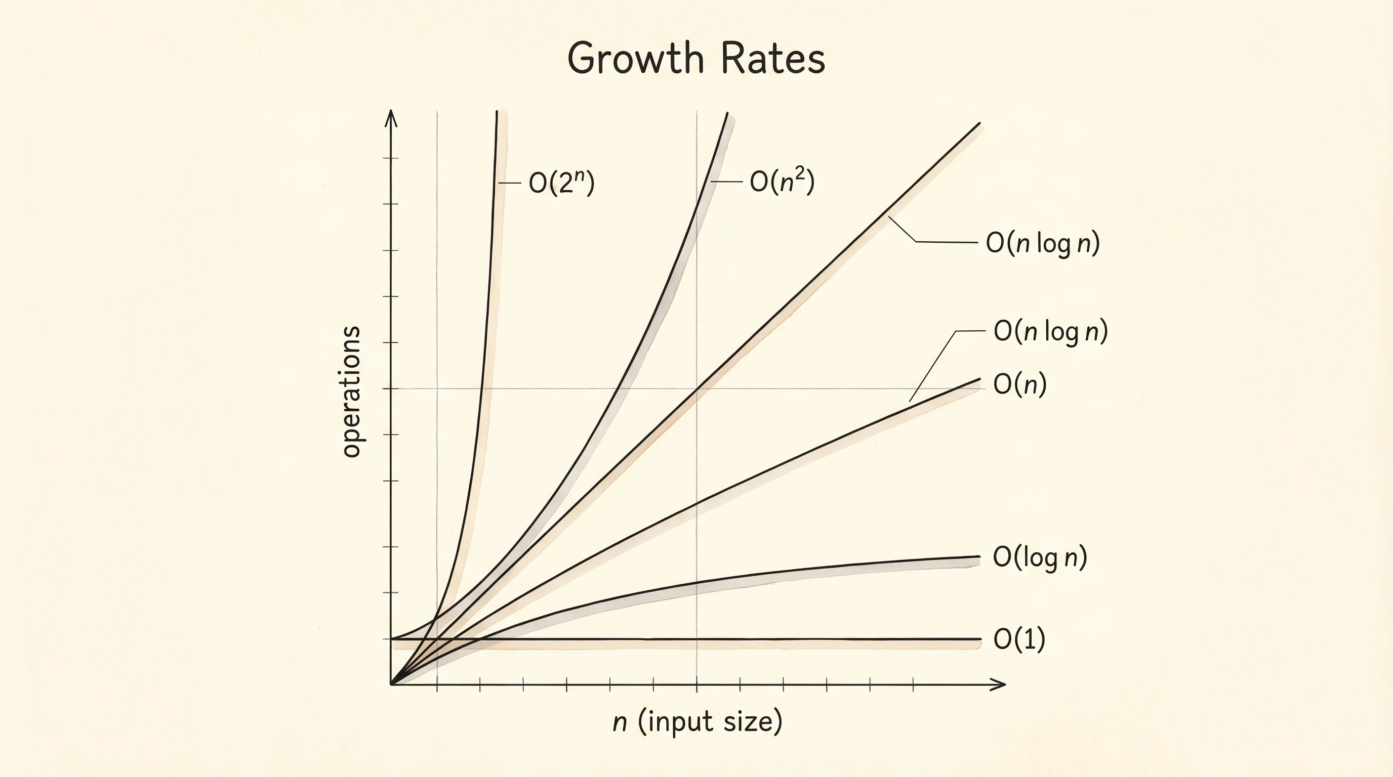
The vocabulary is small. O(1) is constant: the work does not grow at all. Looking up nums[5] in a Python list takes the same time whether the list has 10 items or 10 million. O(log n) is logarithmic: the work grows but slowly. Each time the input doubles, the work goes up by one step. O(n) is linear: double the input and the work doubles. O(n log n) is linearithmic: a linear pass that does a logarithmic amount of work at each step — the cost of a good sort. O(n^2) is quadratic: double the input and the work goes up by 4. O(2^n) is exponential: add one to the input and the work doubles. O(n!) is factorial: this is what happens when you try every permutation of a set. The last two get unrunnable fast.

A table grounds it. For an input of size 100 vs 1000, here is what each class costs in operations.

n = 100      n = 1000
O(1)            1            1
O(log n)        7           10
O(n)          100         1000
O(n log n)    700        10000
O(n^2)      10000      1000000
O(2^n)    2^100        2^1000   (don't run these)

You do not need to memorize the table. You need to feel the gap. Going from O(n) to O(n^2) at n=1000 is the difference between 1000 operations and a million. At n=10000 it is 10000 vs 100 million. The squared row beats your patience long before it beats your laptop.

Numbers on a page are theory. Real time on a real machine is the proof. Open bigo.py in the venv and write a tiny tool — a decorator that wraps any function and prints how long it took. A decorator is a function that takes a function and gives you a new one with extra behavior. We will properly cover decorators later. For now, type it and watch it work.

import time
from typing import Callable
 
def timer(fn: Callable) -> Callable:
    def wrapped(*args, **kwargs):
        start = time.perf_counter()
        result = fn(*args, **kwargs)
        elapsed = time.perf_counter() - start
        print(f"{fn.__name__}({len(args[0])}) took {elapsed * 1000:.3f} ms")
        return result
    return wrapped
 
@timer
def linear_search(nums, target):
    for i, value in enumerate(nums):
        if value == target:
            return i
    return -1
 
for size in [10, 100, 1000, 10000, 100000]:
    nums = list(range(size))
    linear_search(nums, -1)

The function we are timing is the dumbest possible search: walk every element until you find the target. We always pass -1, which is not in the list, so the function always walks the whole thing. That is the worst case for linear search, which is what Big O measures by default. Run it.

linear_search(10) took 0.001 ms
linear_search(100) took 0.005 ms
linear_search(1000) took 0.046 ms
linear_search(10000) took 0.470 ms
linear_search(100000) took 4.621 ms

Look at the rightmost numbers. Each time the input goes up by 10, the time goes up by 10. That is O(n) staring back at you in milliseconds. The machine confirms what the formula promised. If the function were O(n^2) the times would have grown by 100 each row, and the last line would have been seconds, not milliseconds.

Now make it visible. Plotly is a charting library that draws interactive graphs in your browser. It is the one library we import in this lesson because drawing is not the same as logic — we are not asking Plotly to do the algorithm, only to render the numbers we already collected. Install it once:

pip install plotly

pip install plotly

import plotly.graph_objects as go
 
sizes = [10, 100, 1000, 10000, 100000]
times_ms = [0.001, 0.005, 0.046, 0.470, 4.621]
 
fig = go.Figure()
fig.add_trace(go.Scatter(x=sizes, y=times_ms, mode="lines+markers", name="linear search"))
fig.update_layout(
    title="Linear search runtime vs input size",
    xaxis_title="n",
    yaxis_title="milliseconds",
    xaxis_type="log",
    yaxis_type="log",
)
fig.show()

The chart opens in your browser. On a log-log plot a linear function shows up as a straight line at 45 degrees. A quadratic function shows up as a steeper line. An exponential function curves up off the page. You can eyeball the class of an algorithm from this kind of plot once you have run it on a few sizes.

A note on best, worst, and average case. Linear search is O(n) worst case — the target is at the end. It is O(1) best case — the target is the first element. The average over random positions is O(n/2), which Big O writes as O(n) because constants do not matter in the limit. When someone says "this is O(n^2)" without qualifying, they mean worst case. That is the conservative number, the one you plan for.

You have a vocabulary now and a way to measure. The next move is to take a list that someone handed you in any order and put it in the order you actually want.