Graphs

A city map is the last shape. Intersections are the nodes — vertices, in the formal vocabulary. Roads are the edges. There is no root, no parent, no left or right child. From any intersection you can drive in several directions, and the road might come back on itself, fork, or rejoin a street you were on three blocks ago. The map is a graph. Once you have one, you can ask the question every navigation app exists to answer: what is the shortest sequence of roads from where I am to where I want to be?

Graph theory was born from a real city. In 1736 the Swiss mathematician Leonhard Euler was sent a puzzle from Königsberg, a Prussian town crisscrossed by the Pregel River and connected by seven bridges. The townspeople wanted to know whether they could take an evening walk that crossed every bridge exactly once and ended where they started. Euler reframed the map: collapse each landmass into a single dot, draw a line for each bridge, and ignore the geography. He then proved no such walk existed because four of the dots had an odd number of bridges attached, and in any such tour every dot except the start and end must have an even count. The proof was the first paper in graph theory and the moment a city map became a math object. Two centuries later Edsger Dijkstra was sitting in an Amsterdam coffee shop in 1956, trying to demonstrate the new ARMAC computer. He picked the problem of the shortest route from Rotterdam to Groningen, designed an algorithm in 20 minutes without writing it down, and only published it in 1959. The algorithm is still the one your phone runs every time it routes you home. Then in 1998 two Stanford grad students named Larry Page and Sergey Brin treated the entire web as a graph — pages as vertices, hyperlinks as edges — and ranked pages by how many links pointed at them, weighted by how trustworthy each linker was. PageRank built Google.

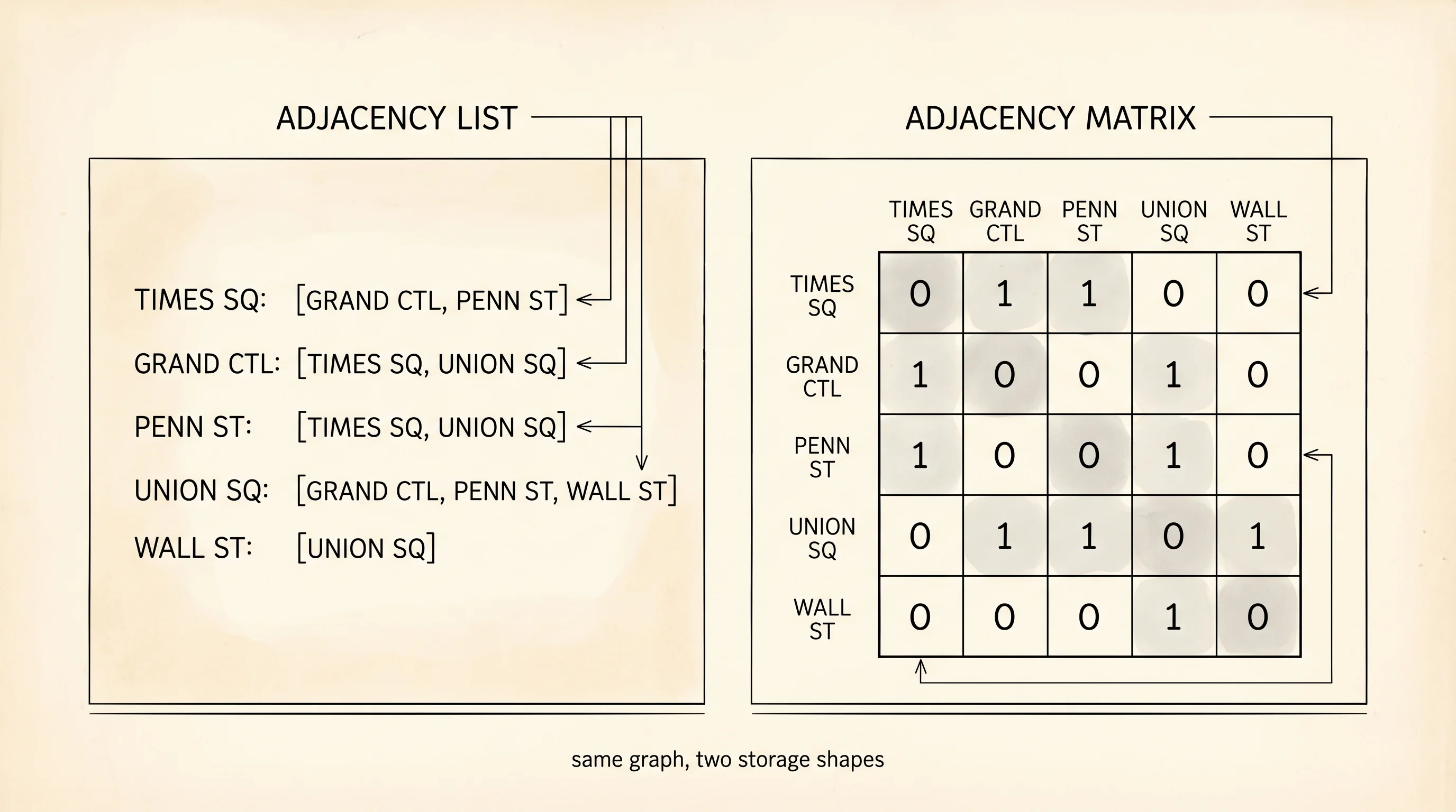
There are two natural ways to write a graph in code. The adjacency matrix is a square table where row i, column j is 1 if there is an edge from vertex i to vertex j and 0 otherwise. It is fast to ask "is there an edge between A and B?" — one lookup. It wastes space when the graph is sparse, because most cells are zero. The adjacency list does the opposite: for each vertex, store a list of its neighbors. It uses memory proportional to the number of edges, not the square of the number of vertices, which is why every real graph library — your phone's GPS, every social network, every AI route planner — uses the list form. Build it in graph.py.

class Graph:
    def __init__(self):
        self.adj = {}
 
    def add_vertex(self, name):
        if name not in self.adj:
            self.adj[name] = []
 
    def add_edge(self, a, b):
        self.add_vertex(a)
        self.add_vertex(b)
        if b not in self.adj[a]:
            self.adj[a].append(b)
        if a not in self.adj[b]:
            self.adj[b].append(a)
 
    def neighbors(self, name):
        return list(self.adj.get(name, []))
 
    def show(self):
        for vertex in self.adj:
            print(f"  {vertex}: {self.adj[vertex]}")
        print()

The graph is undirected — every edge goes both ways, so when you connect A and B, A's neighbor list gets B and B's gets A. The show method prints the whole adjacency list. Add a few intersections and watch the city take shape.

g = Graph()
print("--- empty ---")
g.show()
 
for a, b in [
    ("Times Square", "Grand Central"),
    ("Times Square", "Penn Station"),
    ("Grand Central", "Union Square"),
    ("Penn Station", "Union Square"),
    ("Union Square", "Wall Street"),
]:
    print(f"--- after add_edge({a!r}, {b!r}) ---")
    g.add_edge(a, b)
    g.show()

Output:

--- empty ---
 
--- after add_edge('Times Square', 'Grand Central') ---
  Times Square: ['Grand Central']
  Grand Central: ['Times Square']
 
--- after add_edge('Times Square', 'Penn Station') ---
  Times Square: ['Grand Central', 'Penn Station']
  Grand Central: ['Times Square']
  Penn Station: ['Times Square']
 
--- after add_edge('Grand Central', 'Union Square') ---
  Times Square: ['Grand Central', 'Penn Station']
  Grand Central: ['Times Square', 'Union Square']
  Penn Station: ['Times Square']
  Union Square: ['Grand Central']
 
--- after add_edge('Penn Station', 'Union Square') ---
  Times Square: ['Grand Central', 'Penn Station']
  Grand Central: ['Times Square', 'Union Square']
  Penn Station: ['Times Square', 'Union Square']
  Union Square: ['Grand Central', 'Penn Station']
 
--- after add_edge('Union Square', 'Wall Street') ---
  Times Square: ['Grand Central', 'Penn Station']
  Grand Central: ['Times Square', 'Union Square']
  Penn Station: ['Times Square', 'Union Square']
  Union Square: ['Grand Central', 'Penn Station', 'Wall Street']
  Wall Street: ['Union Square']

Read top to bottom. Each new edge shows up in two places — once in each endpoint's neighbor list, because the edge is undirected. Union Square is the busiest node by the end, with three neighbors. Wall Street is the loneliest with one. Calling g.neighbors("Union Square") returns ['Grand Central', 'Penn Station', 'Wall Street'] — exactly the streets you can drive to from there in one hop.

The matrix view exists too. For five vertices, build a 5×5 grid and put a 1 wherever an edge exists.

def adjacency_matrix(g):
    names = list(g.adj.keys())
    index = {name: i for i, name in enumerate(names)}
    n = len(names)
    matrix = [[0] * n for _ in range(n)]
    for vertex, neighbors in g.adj.items():
        i = index[vertex]
        for neighbor in neighbors:
            j = index[neighbor]
            matrix[i][j] = 1
 
    header = "      " + " ".join(name[:3] for name in names)
    print(header)
    for name, row in zip(names, matrix):
        print(f"{name[:3]:>4}  " + " ".join(f"{cell:>3}" for cell in row))
 
adjacency_matrix(g)

Output:

      Tim Gra Pen Uni Wal
 Tim    0   1   1   0   0
 Gra    1   0   0   1   0
 Pen    1   0   0   1   0
 Uni    0   1   1   0   1
 Wal    0   0   0   1   0

Same graph, two shapes. The matrix is symmetric across the diagonal because the graph is undirected. The diagonal is all zeros because there are no self-loops. Counting the 1s above the diagonal gives the edge count: 5. With five vertices the matrix has 25 cells and only 10 of them are 1s (each edge appears twice). For a city with 10,000 intersections the matrix would have 100 million cells. The adjacency list, by contrast, would be a few million pointers. The list wins on every realistic graph.

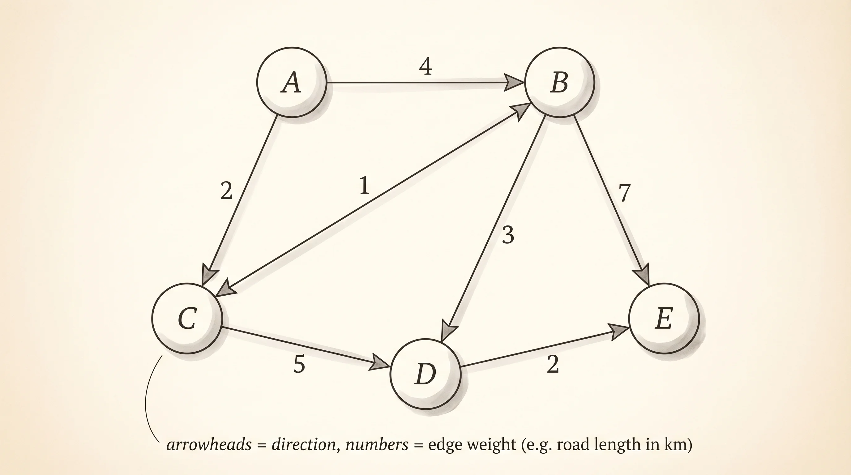
Directed graphs only put the edge in one direction's neighbor list, which models one-way streets, Twitter follows, and every web hyperlink. Weighted graphs replace each neighbor with a (neighbor, weight) pair, which models distances, costs, or capacities — the data Dijkstra's 1956 algorithm walks to find shortest paths.

Now the Act-2 reach. Python has no built-in graph type because the language is happy to let you use a dict of lists directly. The class you wrote is mostly bookkeeping over a dict[str, list[str]]. Type the same edges into a raw dict and watch the structure look identical.

city = {}
for a, b in [
    ("Times Square", "Grand Central"),
    ("Times Square", "Penn Station"),
    ("Grand Central", "Union Square"),
    ("Penn Station", "Union Square"),
    ("Union Square", "Wall Street"),
]:
    city.setdefault(a, []).append(b)
    city.setdefault(b, []).append(a)
 
for vertex, neighbors in city.items():
    print(f"  {vertex}: {neighbors}")

Output:

  Times Square: ['Grand Central', 'Penn Station']
  Grand Central: ['Times Square', 'Union Square']
  Penn Station: ['Times Square', 'Union Square']
  Union Square: ['Grand Central', 'Penn Station', 'Wall Street']
  Wall Street: ['Union Square']

Identical adjacency list. The setdefault trick gives you the "create the list on first touch" behavior the Graph class hid behind add_vertex. For production work people still write a Graph class because it gives you a place to attach methods like shortest_path and connected_components, but the storage underneath is always some flavor of dict[str, list]. The big serious libraries — NetworkX in Python, igraph in C, Apache Giraph for distributed graphs — all wrap the same idea.

Question: in the city graph above, how many one-hop trips exist that start at Union Square?

Answer: three. The neighbors list says ['Grand Central', 'Penn Station', 'Wall Street'], so from Union Square you can ride one stop to any of those three stations.

You now have every shape the rest of the curriculum needs: ordered rows, chains, stacks, lines, named lookups, hierarchies, and now networks. Containers hold the data. The next section is the recipes that walk through them — sorting them, searching them, finding the cheapest route from one node to another. The shapes were the noun. The algorithms are the verbs.