Trees
The library has one more shape hidden in plain sight. Walk the building and read the wall signs. Floor 1 is split into Fiction and Non-Fiction. Non-Fiction breaks into Science, History, and Arts. Science breaks into Biology, Physics, Chemistry. Biology breaks into Botany and Zoology. Each sign sits above a smaller set of signs, which sit above an even smaller set. The whole building is a tree. The classification scheme — Melvil Dewey published it in 1876 — is the same shape that sits inside every database, every filesystem, every JSON document, and every chess engine. A node sits at the top, fans out to children, who fan out to grandchildren, and so on until you hit a shelf with the actual books. Computer scientists call the top a root and the books leaves, even though that flips the metaphor upside down.
The shape was on paper long before computers. Jan Łukasiewicz at the University of Warsaw wrote logical formulas in 1924 in a parenthesis-free notation that turned out to be a tree walk in disguise. The big arrival was 1971 at Boeing's research lab in Seattle: Rudolf Bayer and Edward McCreight published the B-tree, designed to fit a database index into a stack of disk pages with as few seeks as possible. Every relational database since — Oracle, MySQL, Postgres, SQLite — keeps its primary indexes as some flavor of B-tree. Every time a SQL SELECT ... WHERE id = 47 returns in a millisecond instead of scanning a million rows, it is walking a tree from the root, with each hop eliminating roughly half the remaining rows. The binary search tree you are about to build is the simpler ancestor of that idea.
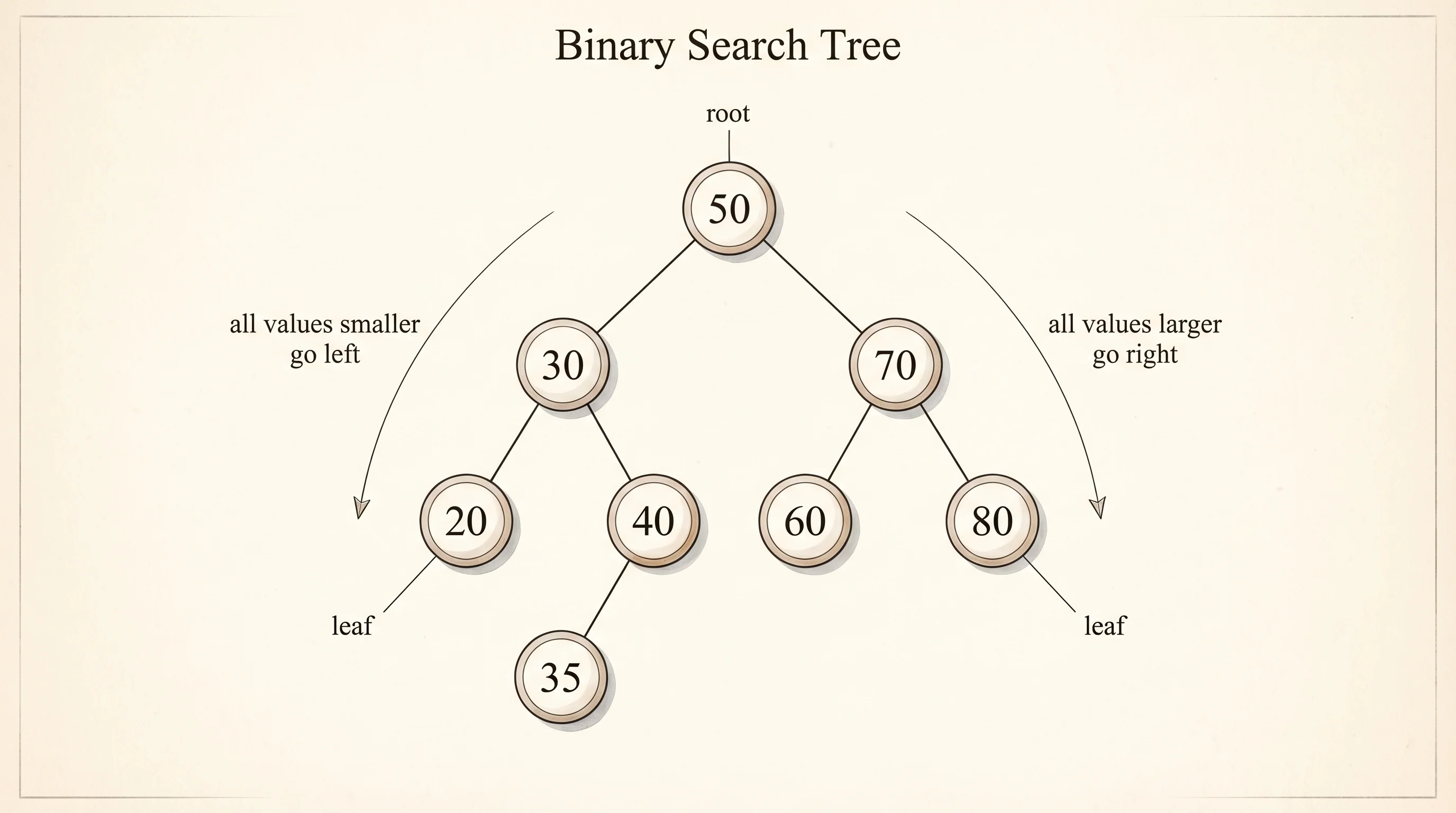
A binary search tree puts one rule on the structure: every node has at most two children, and for any node, all values in its left subtree are smaller and all values in its right subtree are larger. That rule is the entire trick. To find a value, start at the root and ask: smaller, larger, or equal? Step left, right, or stop. Each step throws away half the remaining tree. To insert a new value, walk down with the same rule and tuck the new node into the first empty slot. Build it in bst.py.
class TreeNode:
    def __init__(self, value):
        self.value = value
        self.left = None
        self.right = None


class BST:
    def __init__(self):
        self.root = None

    def insert(self, value):
        self.root = self._insert(self.root, value)

    def _insert(self, node, value):
        if node is None:
            return TreeNode(value)
        if value < node.value:
            node.left = self._insert(node.left, value)
        elif value > node.value:
            node.right = self._insert(node.right, value)
        return node

    def search(self, value):
        node = self.root
        while node is not None:
            if value == node.value:
                return True
            node = node.left if value < node.value else node.right
        return False

    def inorder(self):
        result = []
        self._inorder(self.root, result)
        return result

    def _inorder(self, node, result):
        if node is None:
            return
        self._inorder(node.left, result)
        result.append(node.value)
        self._inorder(node.right, result)

    def preorder(self):
        result = []
        self._preorder(self.root, result)
        return result

    def _preorder(self, node, result):
        if node is None:
            return
        result.append(node.value)
        self._preorder(node.left, result)
        self._preorder(node.right, result)

    def show(self):
        lines = []
        self._draw(self.root, "", True, lines)
        print("\n".join(lines) if lines else "(empty)")

    def _draw(self, node, prefix, is_tail, lines):
        if node is None:
            return
        connector = "+-- " if is_tail else "|-- "
        lines.append(prefix + connector + str(node.value))
        new_prefix = prefix + ("    " if is_tail else "|   ")
        children = [(node.left, "L"), (node.right, "R")]
        children = [c for c in children if c[0] is not None]
        for i, (child, _label) in enumerate(children):
            self._draw(child, new_prefix, i == len(children) - 1, lines)
The show method prints the tree as ASCII with branch connectors so you can watch the shape grow as values arrive. Insert eight values and call it after each one.
bst = BST()
for value in [50, 30, 70, 20, 40, 60, 80, 35]:
    bst.insert(value)
    print(f"--- after inserting {value} ---")
    bst.show()
Output:
--- after inserting 50 ---
+-- 50
--- after inserting 30 ---
+-- 50
    +-- 30
--- after inserting 70 ---
+-- 50
    +-- 30
    +-- 70
--- after inserting 20 ---
+-- 50
    +-- 30
    |   +-- 20
    +-- 70
--- after inserting 40 ---
+-- 50
    +-- 30
    |   +-- 20
    |   +-- 40
    +-- 70
--- after inserting 60 ---
+-- 50
    +-- 30
    |   +-- 20
    |   +-- 40
    +-- 70
        +-- 60
--- after inserting 70 ---
... (above plus the rest)
50 is the root. 30 went left because 30 < 50. 70 went right. 20 walked left from 50, then left from 30 again, and slotted in. The shape grows by following the rule.
Once the tree exists, the interesting move is how you walk through every node. There are three classical orders, all variants of "do something at each node, then recurse left and right, in some order."
print("inorder (left, self, right):", bst.inorder())
print("preorder (self, left, right):", bst.preorder())
Output:
inorder (left, self, right): [20, 30, 35, 40, 50, 60, 70, 80]
preorder (self, left, right): [50, 30, 20, 40, 35, 70, 60, 80]
Read the inorder list. It is sorted. That is the magic of a BST — an inorder traversal is a free sort, because the rule "smaller on the left, larger on the right" is exactly what sortedness means. Preorder visits the root first, then descends into the left subtree before the right. That order is what you want when you are saving the tree to disk or copying its shape, because writing down the root before its children lets you rebuild from the top.
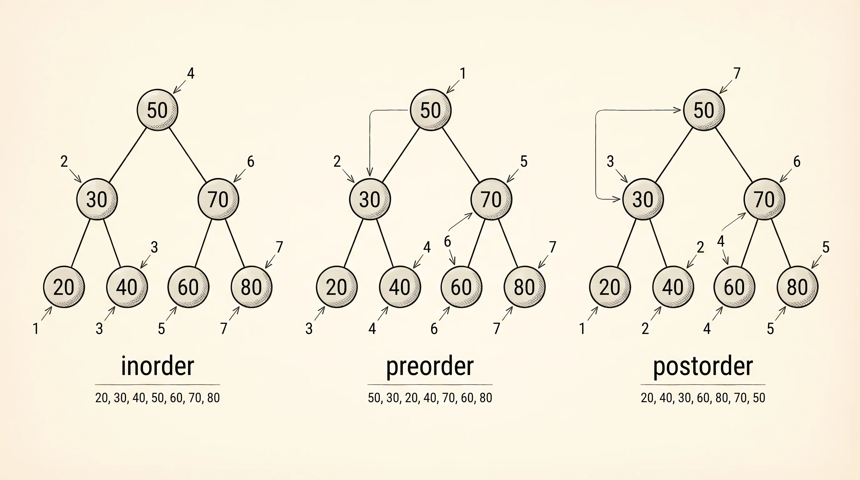
The catch with a hand-rolled BST is balance. Insert values in already-sorted order — 1, 2, 3, 4, 5 — and every node will go right with no left children. The tree degenerates into a chain, and search collapses from O(log n) back to O(n). Production trees keep themselves balanced after each insert: AVL trees from 1962, red-black trees from 1972, B-trees from 1971, all of which add bookkeeping to maintain a good shape. Python's standard library does not ship a tree class. What it does ship is bisect, which gets you most of the practical benefit by maintaining a sorted list and using binary search to find positions in O(log n) lookup time, with the cost of O(n) inserts.
import bisect

sorted_list = []
for value in [50, 30, 70, 20, 40, 60, 80, 35]:
    bisect.insort(sorted_list, value)
    print(f"after insert {value}: {sorted_list}")

idx = bisect.bisect_left(sorted_list, 40)
print(f"40 is at index {idx}")
print(f"in list? {sorted_list[idx] == 40}")
Output:
after insert 50: [50]
after insert 30: [30, 50]
after insert 70: [30, 50, 70]
after insert 20: [20, 30, 50, 70]
after insert 40: [20, 30, 40, 50, 70]
after insert 60: [20, 30, 40, 50, 60, 70]
after insert 80: [20, 30, 40, 50, 60, 70, 80]
after insert 35: [20, 30, 35, 40, 50, 60, 70, 80]
40 is at index 3
in list? True
Notice the final bisect.insort produced the same sequence as the BST's inorder traversal. That is not a coincidence. Both structures encode the same sorted order, with different tradeoffs on insert and search cost. bisect is what reach for in everyday Python code when you need a sorted collection. The BST you wrote is what the runtime is doing when you reach for a relational database index.
Question: in the BST insertion trace, why did 35 end up to the right of 30 and to the left of 40, instead of becoming a child of 50 directly?
Answer: the insert walks from the root using the rule. 35 < 50 so it goes left. 35 > 30 so it goes right of 30. 35 < 40 so it goes left of 40. The first empty slot it finds is the left child of 40, and that is where it lands.
A tree captures a hierarchy — every node has one parent. Sometimes the world is messier. A subway map has stations that connect to several other stations, with no single root and no parent-child rule. When the relationships fan out in every direction, you need a shape with no ranks at all.