Vectors and Matrices
A neural network is a tower of multiplications. Before you can build the tower, you need the steel it is welded from. The steel is two ideas: a vector, which is a point in space, and a matrix, which is a rule for moving every point in space at once. The next 43 lessons forge a brain out of pure Python. The first thing the workshop opens with is the bench where the steel is rolled.
The math was written down before any computer existed. Arthur Cayley and James Joseph Sylvester, two friends who met as young lawyers in London in 1850, kept passing each other notes about square arrays of numbers and the rules for multiplying them. Cayley wrote the first paper on matrices in 1858. Nobody used them for anything practical for the next 60 years. In 1925 a 23-year-old Werner Heisenberg, recovering from hay fever on the island of Helgoland, sat down to work out the energies of a hydrogen atom and ended up multiplying tables of numbers in an order that did not commute — A times B did not equal B times A. He showed it to his teacher Max Born, who took one look and told him: those are matrices. The thing Heisenberg had reinvented from physics was the same thing Cayley had written down for fun. Half a century later, in 1976, Gilbert Strang at MIT started teaching 18.06 the way programmers needed it: every concept tied to a small numerical example you could compute by hand. His textbook is the reason most working engineers know the subject. And every modern deep learning framework — PyTorch, TensorFlow, JAX — spends 90 percent of its runtime inside a single function called matmul, the matrix multiply. Learn this one operation and you have learned what the GPU is doing.
A vector in 2D is two numbers, an x and a y. Picture a flat sheet of graph paper with the origin in the middle. The vector (3, 2) is the arrow from the origin to the dot at column 3, row 2. Add two vectors and you get a third — slide one arrow to the tip of the other. Multiply a vector by a number and the arrow stretches or shrinks. Open a file called geometry.py and type a class for it.
import math


class Vector2D:
    def __init__(self, x, y):
        self.x = x
        self.y = y

    def __repr__(self):
        return f"({self.x:.2f}, {self.y:.2f})"

    def __add__(self, other):
        return Vector2D(self.x + other.x, self.y + other.y)

    def scale(self, k):
        return Vector2D(self.x * k, self.y * k)

    def dot(self, other):
        return self.x * other.x + self.y * other.y


a = Vector2D(3, 2)
b = Vector2D(1, 4)
print(a + b)
print(a.scale(2))
print(a.dot(b))
The output reads:
(4.00, 6.00)
(6.00, 4.00)
11.00
The dot product is the one that pays the bills. It is one number — multiply the x components, multiply the y components, add the two products. That single sum is the only operation a neuron ever does. Every weight times every input, all summed. Hold onto that.
A matrix in 2D is four numbers laid out as two rows and two columns. The point of a matrix is not the numbers — it is what happens when you multiply it by a vector. The matrix takes the input vector and spits out a new vector, which is the input moved somewhere else on the plane. Pick the four numbers right and you can rotate every point, scale every point, flip every point, or shear every point, all with the same operation.
class Matrix2x2:
def __init__(self, a, b, c, d):
self.a = a
self.b = b
self.c = c
self.d = d
def __repr__(self):
return f"[[{self.a:.2f}, {self.b:.2f}], [{self.c:.2f}, {self.d:.2f}]]"
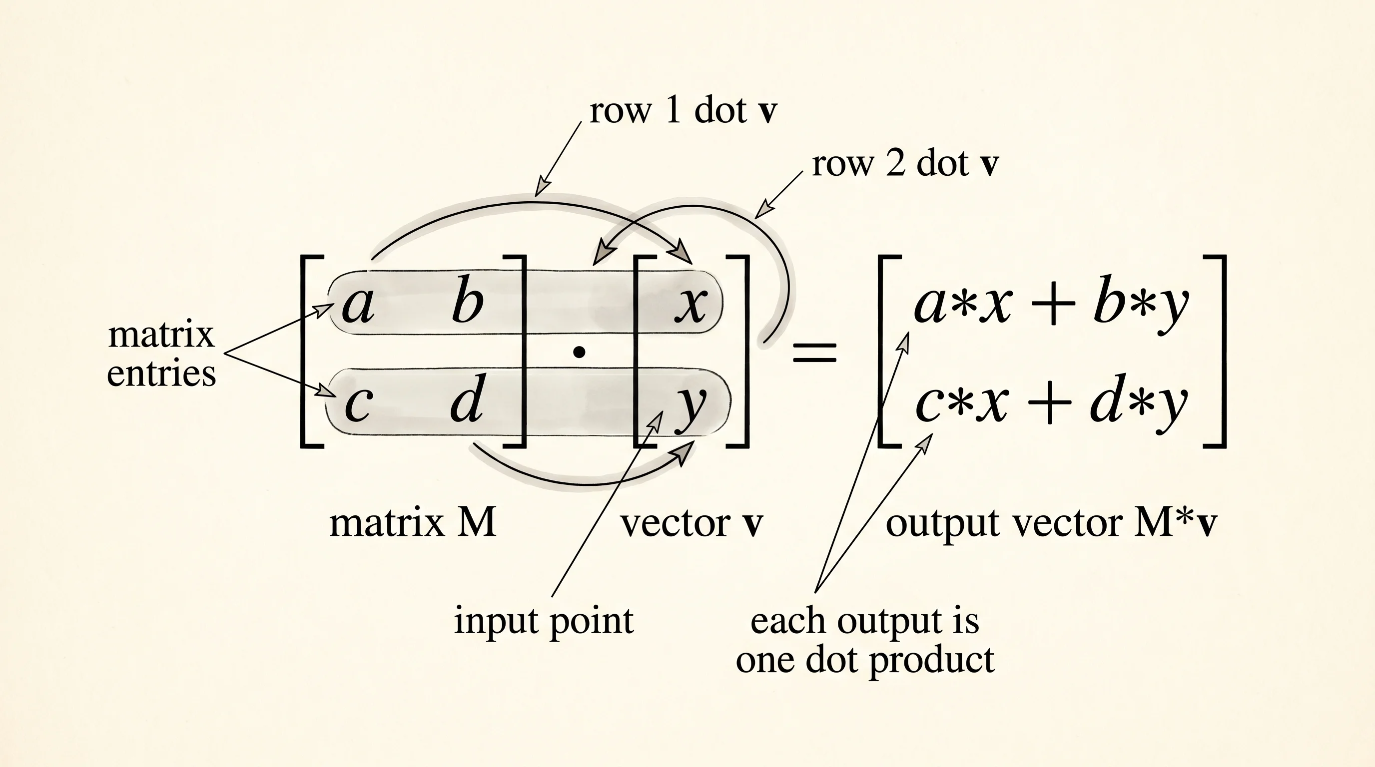
def apply(self, v):
return Vector2D(
self.a * v.x + self.b * v.y,
self.c * v.x + self.d * v.y,
)
def compose(self, other):
return Matrix2x2(
self.a * other.a + self.b * other.c,
self.a * other.b + self.b * other.d,
self.c * other.a + self.d * other.c,
self.c * other.b + self.d * other.d,
)The apply method is the matrix-vector multiply: row 1 of the matrix dotted with the vector gives the new x, row 2 dotted with the vector gives the new y. Two dot products. The compose method is the matrix-matrix multiply: it builds one new matrix that does the work of two matrices in a row. Compose is what makes neural networks deep — stack 12 matrices and the composition is one matrix that already knows the path through all 12.
The famous transformations are short recipes for these four numbers. A rotation by angle theta is [[cos, -sin], [sin, cos]]. A scale by sx in x and sy in y is [[sx, 0], [0, sy]]. A reflection across the x-axis flips the sign of y, so it is [[1, 0], [0, -1]]. Add these as factory functions in the same file.
def rotation(angle_radians):
c = math.cos(angle_radians)
s = math.sin(angle_radians)
return Matrix2x2(c, -s, s, c)
def scale(sx, sy):
return Matrix2x2(sx, 0, 0, sy)
def reflect_x():
return Matrix2x2(1, 0, 0, -1)
def reflect_y():
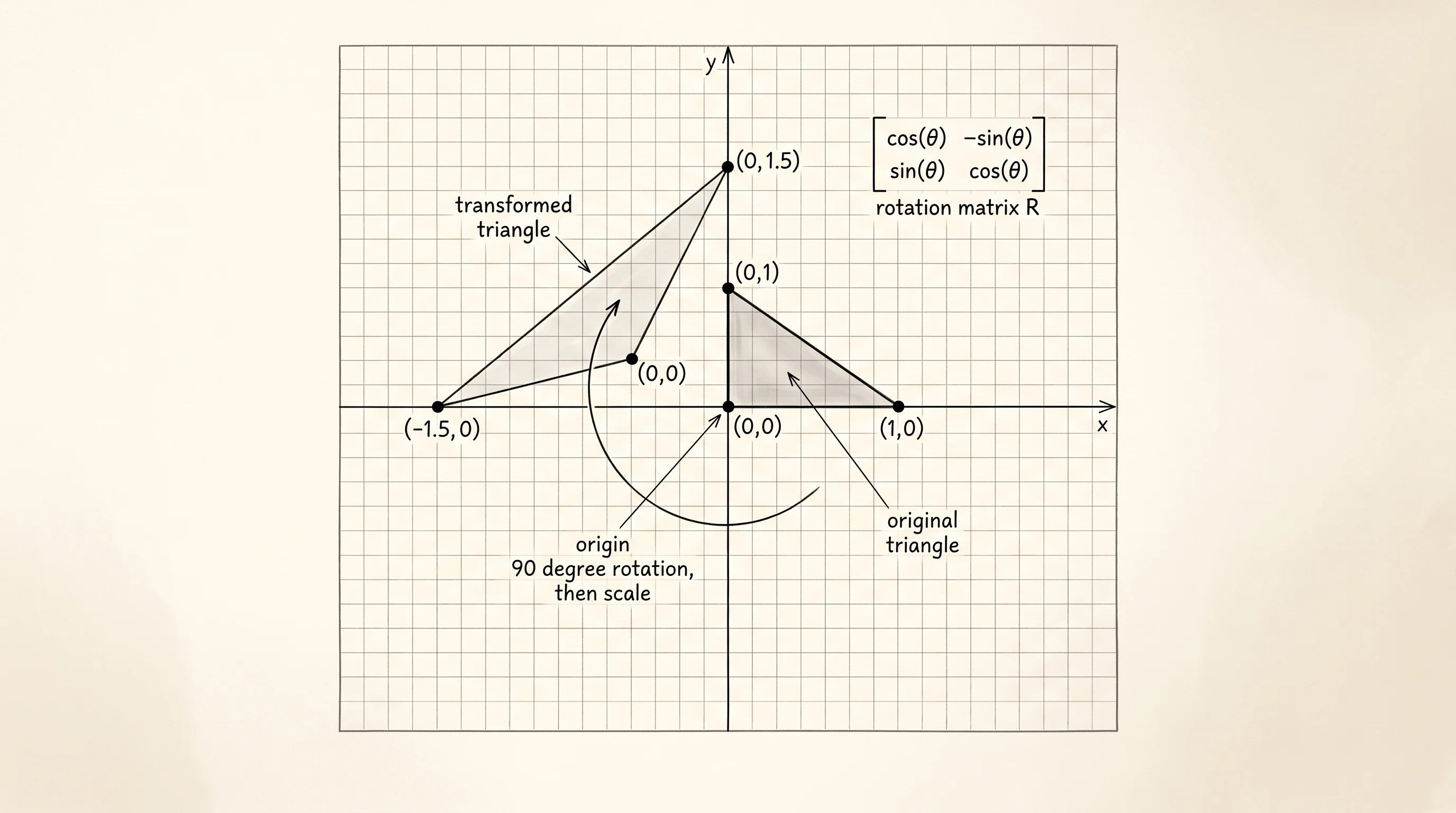
return Matrix2x2(-1, 0, 0, 1)Now build the simplest shape that has a clear orientation: a triangle with three vertices. Print the vertices, rotate them by 90 degrees, print again, then scale by 2 in x, print again, then compose the rotation and the scale into one matrix, apply that, and print the final.
triangle = [Vector2D(1, 0), Vector2D(0, 1), Vector2D(0, 0)]
print("original:    ", triangle)

R = rotation(math.pi / 2)
rotated = [R.apply(v) for v in triangle]
print("rotated 90:  ", rotated)

S = scale(2, 1)
scaled = [S.apply(v) for v in rotated]
print("then scaled: ", scaled)

M = S.compose(R)
both = [M.apply(v) for v in triangle]
print("composed:    ", both)
Run it.
original:     [(1.00, 0.00), (0.00, 1.00), (0.00, 0.00)]
rotated 90:   [(0.00, 1.00), (-1.00, 0.00), (0.00, 0.00)]
then scaled:  [(0.00, 1.00), (-2.00, 0.00), (0.00, 0.00)]
composed:     [(0.00, 1.00), (-2.00, 0.00), (0.00, 0.00)]
The third frame and the fourth frame match exactly. That is the whole reason matrix multiplication exists. The composed matrix M = S times R does in one step what the two earlier steps did in two. Reverse the order — R.compose(S) instead of S.compose(R) — and the answer changes, because rotating then stretching is not the same as stretching then rotating. This is the Heisenberg surprise from 1925, alive on your screen. A small question to answer from the run: which vertex stayed in place across every transformation?
The origin (0, 0). Multiplying any matrix by the zero vector gives the zero vector — every term has a zero in it. The origin is the one fixed point of any rotation, scale, or reflection that goes through these factories.
Numbers in a list are hard to picture. The shape moves in space, so the way to feel it is to draw it. A canvas is a 2D grid of characters you write into and then print. Plot a vertex by putting a * at the right cell. Connect two vertices with a line drawn one cell at a time using Bresenham's algorithm — a 1965 trick by Jack Bresenham at IBM that walks along the longer axis and steps on the shorter axis only when the error has built up enough. Add a Canvas class.
class Canvas:
    def __init__(self, size=21):
        self.size = size
        self.cells = [[" "] * size for _ in range(size)]

    def to_pixel(self, v):
        cx = self.size // 2
        cy = self.size // 2
        return cx + int(round(v.x)), cy - int(round(v.y))

    def plot(self, v, mark="*"):
        x, y = self.to_pixel(v)
        if 0 <= x < self.size and 0 <= y < self.size:
            self.cells[y][x] = mark

    def line(self, v1, v2, mark="."):
        x0, y0 = self.to_pixel(v1)
        x1, y1 = self.to_pixel(v2)
        dx = abs(x1 - x0)
        dy = -abs(y1 - y0)
        sx = 1 if x0 < x1 else -1
        sy = 1 if y0 < y1 else -1
        err = dx + dy
        while True:
            if 0 <= x0 < self.size and 0 <= y0 < self.size:
                if self.cells[y0][x0] == " ":
                    self.cells[y0][x0] = mark
            if x0 == x1 and y0 == y1:
                break
            e2 = 2 * err
            if e2 >= dy:
                err += dy
                x0 += sx
            if e2 <= dx:
                err += dx
                y0 += sy

    def draw_triangle(self, verts):
        self.line(verts[0], verts[1])
        self.line(verts[1], verts[2])
        self.line(verts[2], verts[0])
        for v in verts:
            self.plot(v, "*")

    def render(self):
        return "\n".join("".join(row) for row in self.cells)
Use a bigger triangle so the shape is visible on the grid, draw three frames — original, rotated, composed — and print them side by side.
big = [Vector2D(6, 0), Vector2D(0, 6), Vector2D(-4, -4)]

c1 = Canvas(21)
c1.draw_triangle(big)

R = rotation(math.pi / 2)
rotated = [R.apply(v) for v in big]
c2 = Canvas(21)
c2.draw_triangle(rotated)

S = scale(2, 1)
M = S.compose(R)
moved = [M.apply(v) for v in big]
c3 = Canvas(21)
c3.draw_triangle(moved)

print("original:")
print(c1.render())
print("\nrotated 90 degrees:")
print(c2.render())
print("\nrotated then scaled in x:")
print(c3.render())
Each render is a 21x21 grid of characters with the triangle visible as * corners and . edges. The first frame points up and to the right. The second frame is the same triangle turned 90 degrees counterclockwise — the corner that was on the right is now on top. The third frame is the rotated triangle stretched horizontally so the same shape now reaches farther across the grid. One line of code did the move. The matrix M carries the entire instruction.
Stack four matrices, each 2x2, and the composition is still one 2x2 matrix that does the same work. That is the deep learning trick written small. A neural network layer is a matrix-vector multiply — one weight matrix multiplied against the input vector to produce the next vector. A 12-layer network is 12 matrices. Training a network is the act of nudging the numbers inside each matrix until the chain of multiplications spits out the answer you want. The reason GPUs run deep learning so fast is that thousands of these multiplications are happening in parallel across thousands of cores. Cayley wrote the rules in a London study. The GPU follows them a trillion times a second.
You can move shapes in space. Now you need to know how things change.