Derivatives and the Chain Rule

The vectors and matrices from last lesson move shapes around. They cannot tell you how fast anything is moving, or which way to nudge a knob to make an answer better. The second material in the workshop is calculus. A derivative is the answer to one question — if I tap this dial a hair to the right, how much does the output move? Every weight in every neural network is a knob, and the derivative is the number the trainer reads off the dial. The chain rule is the trick that lets you read a knob even when it sits five rooms away from the output.

Isaac Newton wrote down the rules first, in a plague-year notebook in 1665, then refused to publish for 22 years because he was worried about being wrong. Gottfried Leibniz worked it out independently in Germany in the 1670s, published first in 1684, and the two men spent the rest of their lives accusing each other of theft. The Royal Society opened a formal inquiry in 1712 — Newton wrote the report himself and ruled in his own favor. The math from both of them was correct and useful, but neither one could explain why dividing a tiny number by another tiny number gave a real answer. That hole sat open for 140 years until Augustin-Louis Cauchy in Paris pinned down the limit in the 1820s and made the whole thing rigorous. The chain rule itself was named by Joseph-Louis Lagrange in the 1790s, the rule for taking apart a function built out of other functions. Backpropagation, the trick that trains every modern neural network, is the chain rule applied node by node from the output of the network back toward the input. No exceptions. Every gradient you will ever compute is Lagrange's rule running backward through Leibniz's notation.

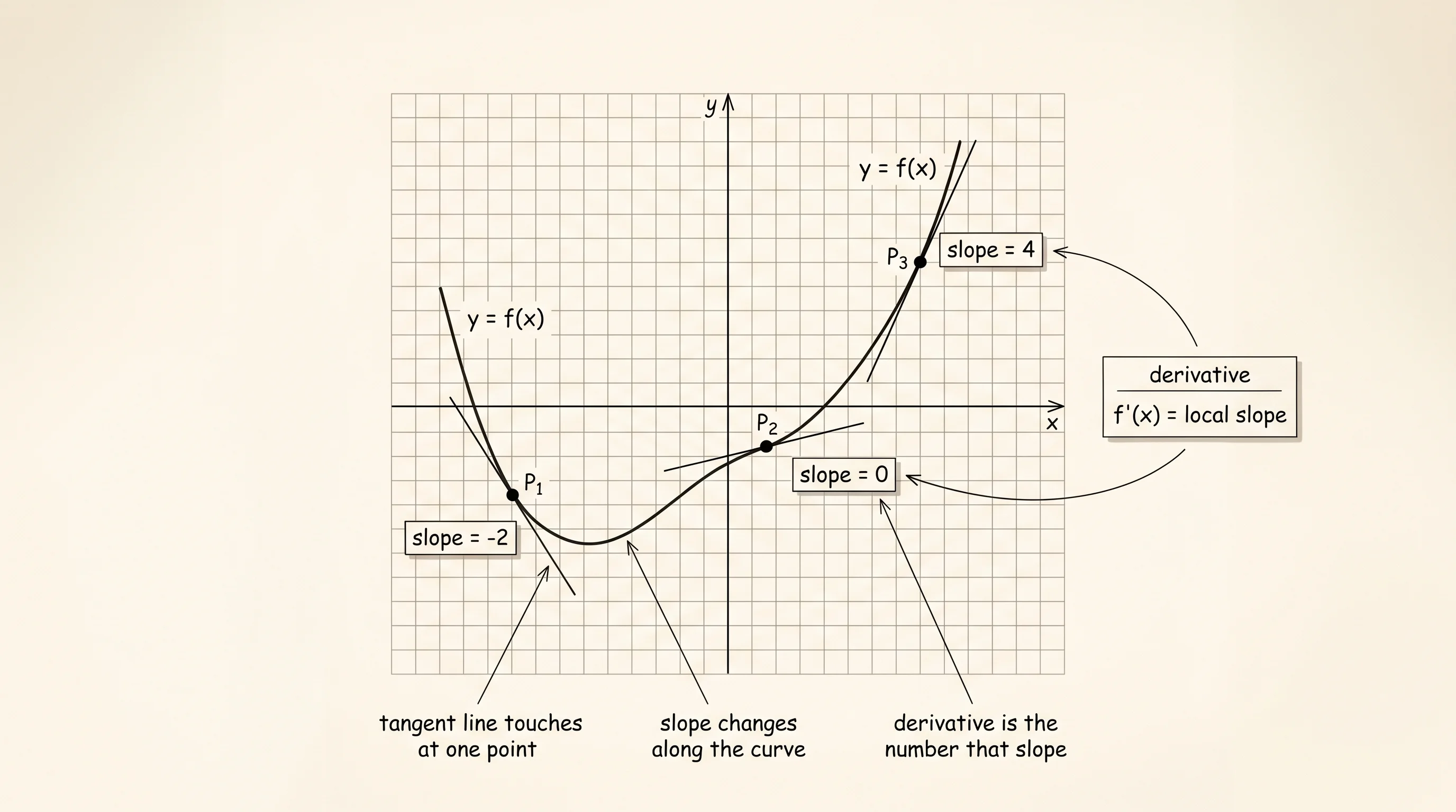
Picture the squat-rack rule from earlier. The weight on the bar is the input. The bar speed off the floor is the output. The derivative is the question you ask the spotter every set: "if I add 5 pounds, how much slower does the bar move?" If the answer is "almost nothing," you add 10 instead. If the answer is "a lot," you back off. The derivative is the local slope of the line you would draw tangent to the curve at the spot you are standing on. Stand at a steep part, the slope is large. Stand at the bottom of a valley, the slope is zero. Newton called this number a fluxion. Leibniz wrote it dy/dx. Modern textbooks write f'(x). All three mean the same thing.

You can compute the derivative two ways. The numerical way is brute force: pick a tiny number h, evaluate f at x+h and at x-h, and divide the difference by 2h. The smaller h gets, the closer the answer gets to the true slope. Try it.

import math
 
def numerical_derivative(f, x, h=1e-7):
    return (f(x + h) - f(x - h)) / (2 * h)
 
print(numerical_derivative(lambda x: x ** 2, 3))
print(numerical_derivative(math.sin, 0))
print(numerical_derivative(math.exp, 1))

Run it.

5.999999990180527
0.9999999999999983
2.7182818285176324

The slope of x² at x=3 is 6, the slope of sine at 0 is 1, the slope of e^x at 1 is e itself. The numerical method always works and is always a little wrong — the floating-point math eats some accuracy. The symbolic way is the opposite: never plug in a number, manipulate the formula directly using the rules Newton and Leibniz wrote down. The derivative of x² is 2x. The derivative of sin(x) is cos(x). The derivative of e^x is e^x. No approximation. The price is that you have to teach a computer the rules.

You build a small algebra system. Every expression is a tree. A leaf is either a constant or a variable. An interior node is an operation — add, multiply, raise to a power, sin, cos, exp, log — that holds its children. Open differentiator.py.

from dataclasses import dataclass
 
class Expr:
    pass
 
@dataclass(frozen=True, repr=False)
class Const(Expr):
    value: float
    def show(self): return str(self.value)
 
@dataclass(frozen=True, repr=False)
class Var(Expr):
    name: str
    def show(self): return self.name
 
@dataclass(frozen=True, repr=False)
class Add(Expr):
    left: Expr
    right: Expr
    def show(self): return f"({self.left.show()} + {self.right.show()})"
 
@dataclass(frozen=True, repr=False)
class Mul(Expr):
    left: Expr
    right: Expr
    def show(self): return f"({self.left.show()} * {self.right.show()})"
 
@dataclass(frozen=True, repr=False)
class Pow(Expr):
    base: Expr
    exponent: Expr
    def show(self): return f"({self.base.show()} ^ {self.exponent.show()})"

The expression 3 * x^2 + 2 * x + 1 is the tree Add(Add(Mul(Const(3), Pow(Var('x'), Const(2))), Mul(Const(2), Var('x'))), Const(1)). Ugly to type, perfect for a computer to walk. Build the tree once and the rules know how to take it apart.

The differentiator walks the tree and applies one rule per node type. The derivative of a constant is zero. The derivative of x with respect to x is one, otherwise zero. The derivative of a sum is the sum of derivatives. The derivative of a product is the product rule from your high-school textbook: u times v becomes u' times v plus u times v'. The derivative of base raised to a constant n is n times base to the n minus 1, multiplied by the derivative of the base — that last factor is the chain rule. Add the three trig and exponential rules and you can differentiate anything in the tree.

def differentiate(expr, var):
    if isinstance(expr, Const):
        return Const(0)
    if isinstance(expr, Var):
        return Const(1) if expr.name == var else Const(0)
    if isinstance(expr, Add):
        return Add(differentiate(expr.left, var), differentiate(expr.right, var))
    if isinstance(expr, Mul):
        return Add(
            Mul(differentiate(expr.left, var), expr.right),
            Mul(expr.left, differentiate(expr.right, var)),
        )
    if isinstance(expr, Pow):
        n = expr.exponent.value
        return Mul(
            Mul(Const(n), Pow(expr.base, Const(n - 1))),
            differentiate(expr.base, var),
        )
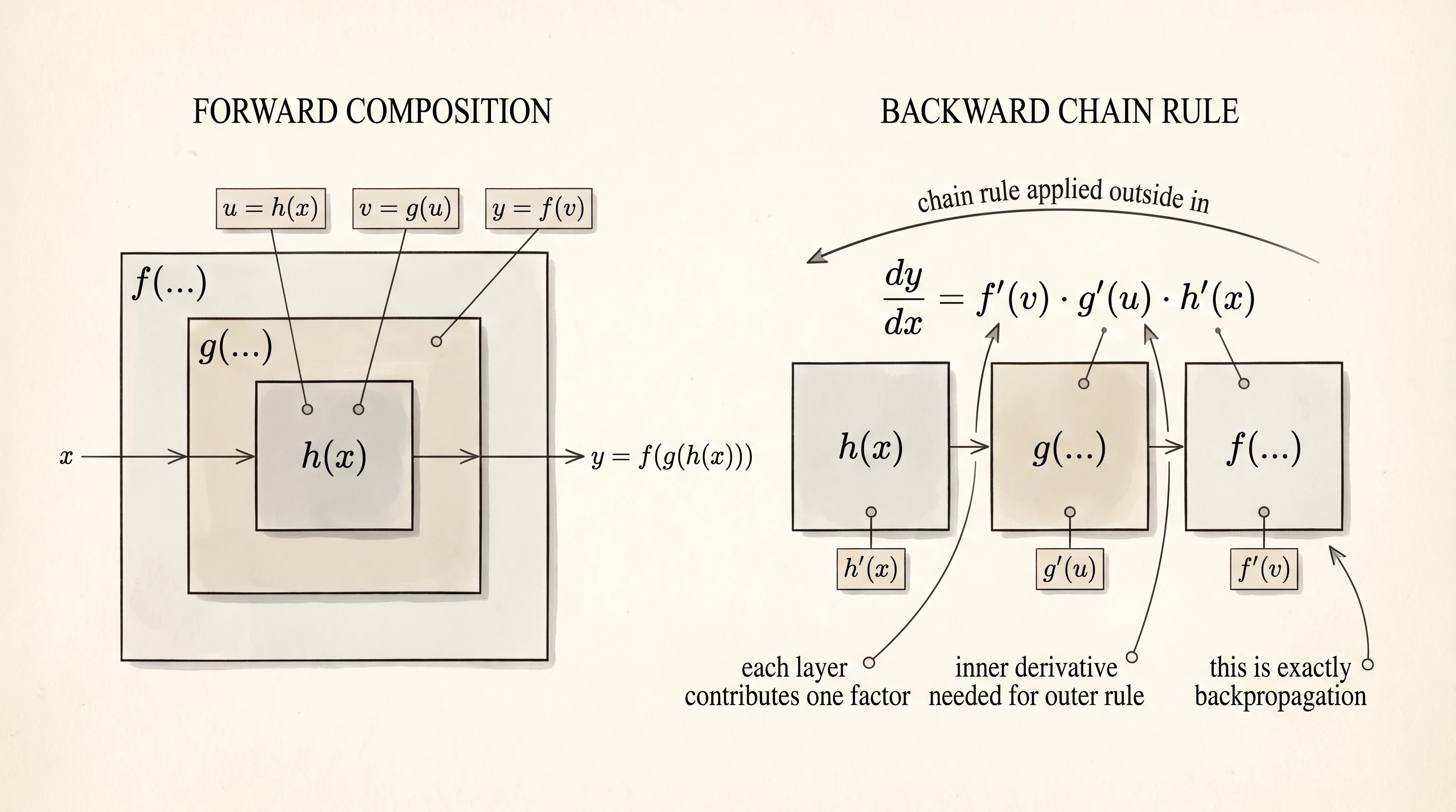
    raise TypeError(type(expr).__name__)

The chain rule shows up inside the Pow case. Pow(sin(x), 2) is sin squared. The derivative is 2 times sin(x) to the 1, times the derivative of sin(x). The function knows nothing about sin — it asks itself "what is the derivative of my base?" and trusts the recursion. That recursive trust is what Lagrange named the chain rule. Read the rule out loud: outer derivative, evaluated at the inner thing, times the derivative of the inner thing. Then repeat at every layer.

The raw derivative tree is correct and unreadable. Every multiply by 1 is still in there. Every add of 0 is still there. Every constant times constant is still in there. Run a simplify pass that walks the tree once more and collapses the obvious cases.

def simplify(expr):
    if isinstance(expr, (Const, Var)):
        return expr
    if isinstance(expr, Add):
        l, r = simplify(expr.left), simplify(expr.right)
        if isinstance(l, Const) and isinstance(r, Const):
            return Const(l.value + r.value)
        if isinstance(l, Const) and l.value == 0: return r
        if isinstance(r, Const) and r.value == 0: return l
        return Add(l, r)
    if isinstance(expr, Mul):
        l, r = simplify(expr.left), simplify(expr.right)
        if isinstance(l, Const) and isinstance(r, Const):
            return Const(l.value * r.value)
        if isinstance(l, Const) and l.value == 0: return Const(0)
        if isinstance(r, Const) and r.value == 0: return Const(0)
        if isinstance(l, Const) and l.value == 1: return r
        if isinstance(r, Const) and r.value == 1: return l
        return Mul(l, r)
    return expr

Add an evaluate that plugs numbers into the tree. It mirrors differentiate — same recursive walk, different operation at each node.

import math
 
def evaluate(expr, bindings):
    if isinstance(expr, Const): return expr.value
    if isinstance(expr, Var): return bindings[expr.name]
    if isinstance(expr, Add):
        return evaluate(expr.left, bindings) + evaluate(expr.right, bindings)
    if isinstance(expr, Mul):
        return evaluate(expr.left, bindings) * evaluate(expr.right, bindings)
    if isinstance(expr, Pow):
        return evaluate(expr.base, bindings) ** evaluate(expr.exponent, bindings)
    raise TypeError(type(expr).__name__)

Now wire it together. Build the polynomial 3x² + 2x + 1, take its derivative, simplify, evaluate the symbolic derivative at three points, and compare each value against the numerical derivative of the original at the same point.

x = Var("x")
f = Add(Add(Mul(Const(3), Pow(x, Const(2))), Mul(Const(2), x)), Const(1))
df = simplify(differentiate(f, "x"))
 
print("f(x)  =", f.show())
print("f'(x) =", df.show())
 
def numerical_derivative(g, x, h=1e-7):
    return (g(x + h) - g(x - h)) / (2 * h)
 
for x_value in [0.5, 1.0, 1.7]:
    symbolic = evaluate(df, {"x": x_value})
    numeric = numerical_derivative(lambda v: evaluate(f, {"x": v}), x_value)
    print(f"x={x_value}: symbolic={symbolic:.6f} numerical={numeric:.6f}")

Run it.

f(x)  = (((3 * (x ^ 2)) + (2 * x)) + 1)
f'(x) = ((3 * (2 * (x ^ 1))) + 2)
x=0.5: symbolic=5.000000 numerical=5.000000
x=1.0: symbolic=8.000000 numerical=8.000000
x=1.7: symbolic=12.200000 numerical=12.200000

A small question for the reader: 3x² + 2x + 1 should differentiate to 6x + 2. The printed derivative reads (3 * (2 * (x ^ 1))) + 2. Did the program get the right answer?

It did. x ^ 1 is x. 3 * (2 * x) is 6x. The simplifier stopped before reducing x ^ 1 to x and before multiplying the two constants. Add two more rules to simplify — one that turns Pow(base, Const(1)) into the base, one that folds Const * (Const * Var) — and the printout reads (6 * x) + 2. Worth doing. Worth not doing in the first pass either — the math is already right and the next lesson does not care about cosmetics.

The full project file is projects/02-symbolic-differentiator/main.py. It has the same shape as what you typed above plus Sin, Cos, Exp, and Log nodes, and it compares against the numerical derivative for five different functions at three points each. The errors are around 1e-9, which is the floor floating-point can give you. Symbolic and numerical agree, every time, to nine decimal places. That agreement is what tells you the rules are right.

The chain rule is what gives a neural network its training signal. A network is a stack of multiplications and activations — exactly the kind of nested function f(g(h(x))) Lagrange wrote about. To know how a weight buried four layers deep affects the final loss, you compute the derivative of the loss with respect to that weight, which by the chain rule is the product of the derivatives at every layer in between. The recursive walk you just wrote is the same shape an autograd engine uses, except autograd records the operations as it runs forward and replays them backward. You will write that engine in lesson 61. The expression tree you built today is the practice rep.

You can compute change. Real data isn't certain. You need a language for uncertainty.