Probability by Simulation
A derivative tells you how the world bends when you nudge it. The world rarely lets you nudge it cleanly. A coin lands heads or tails. A patient tests positive or negative. A roll comes up 4 or 6 or 1. Probability is the third material on the workshop bench: the language for events you cannot predict one at a time but can predict a million at a time. You are not going to learn it from formulas first. You are going to forge it the way the first probabilists did — by rolling dice, counting outcomes, and writing down the number that keeps showing up.
The first person to write a real manual on this was Gerolamo Cardano, a Milanese physician with a serious gambling problem. In 1564 he wrote Liber de Ludo Aleae — "Book on Games of Chance" — to teach himself to lose less money. He worked out that the chance of rolling a particular face on a fair die was 1 in 6 by counting equally likely outcomes. The book sat unpublished for 99 years. The math went mainstream in 1654, when a French nobleman asked Blaise Pascal how to split the pot when a dice game gets cut short. Pascal wrote to Pierre de Fermat. Their letters that summer founded probability theory. A century later, in 1763, a posthumous essay by an English minister named Thomas Bayes was read at the Royal Society. It answered the inverse question — given an outcome, what is the chance it came from a particular cause — and nobody understood how important it was for almost two hundred years. Pierre-Simon Laplace cleaned it up in the early 1800s. Andrey Kolmogorov, in Moscow in 1933, finally axiomatized the whole field on three lines, the way Euclid had done geometry. Every loss function in deep learning today — cross-entropy, KL divergence, log-likelihood — is a direct application of what those four people built.
Start with the smallest engine. A die is an object that, when you ask it for a sample, returns one of six faces with equal chance. Open casino.py in your venv.
import random


class Die:
    def __init__(self, sides=6):
        self.sides = sides

    def sample(self):
        return random.randint(1, self.sides)


d = Die()
for _ in range(10):
    print(d.sample(), end=" ")
print()
Run it. Ten numbers between 1 and 6 in some order. Run it again. Ten different numbers. The output is unpredictable on any single roll. The whole field is built on what happens when you stop looking at single rolls.
Long-run frequency is the first idea. Roll the die a thousand times and count how often each face shows up. Each count, divided by a thousand, is the empirical probability of that face. Add this to casino.py:
def empirical_probabilities(die, n_trials):
    counts = {}
    for _ in range(n_trials):
        face = die.sample()
        counts[face] = counts.get(face, 0) + 1
    return {face: count / n_trials for face, count in counts.items()}


print(empirical_probabilities(Die(), 1000))
print(empirical_probabilities(Die(), 100000))
{1: 0.171, 2: 0.166, 5: 0.169, 6: 0.176, 4: 0.158, 3: 0.16}
{1: 0.16689, 2: 0.16648, 5: 0.16722, 6: 0.16622, 4: 0.16623, 3: 0.16696}At 1,000 trials the numbers wobble around 1/6 (0.1666…) by a percent or two. At 100,000 they hug 1/6 to four decimal places. This is the law of large numbers, and it is the only reason any of probability works. Cardano measured it with his hands. You measured it in 0.04 seconds.
Watch the convergence happen instead of comparing two snapshots. Keep a running mean and print it every 100 rolls.
def running_mean_demo(die, total_trials, print_every=100):
    total = 0
    for trial in range(1, total_trials + 1):
        total += die.sample()
        if trial % print_every == 0:
            print(f"after {trial:>5} rolls: running mean = {total / trial:.4f}")


running_mean_demo(Die(), 2000)
after 100 rolls: running mean = 3.7000
after 200 rolls: running mean = 3.5950
after 300 rolls: running mean = 3.5400
after 400 rolls: running mean = 3.4825
after 500 rolls: running mean = 3.4960
after 600 rolls: running mean = 3.5083
after 700 rolls: running mean = 3.5200
after 800 rolls: running mean = 3.5163
after 900 rolls: running mean = 3.5078
after 1000 rolls: running mean = 3.5070
after 1100 rolls: running mean = 3.5118
after 1200 rolls: running mean = 3.5108
after 1300 rolls: running mean = 3.5100
after 1400 rolls: running mean = 3.5057
after 1500 rolls: running mean = 3.5040
after 1600 rolls: running mean = 3.5006
after 1700 rolls: running mean = 3.4982
after 1800 rolls: running mean = 3.4972
after 1900 rolls: running mean = 3.4967
after 2000 rolls: running mean = 3.4980The first hundred rolls bounce. The next few hundred drift toward 3.5. By 2,000 the running mean has clamped onto 3.5 and stays there. The number 3.5 is the expected value of a fair six-sided die — the average face value, weighted by how often each face shows up. You did not write the formula (1+2+3+4+5+6)/6 = 3.5 to compute it. You measured it. That is the angle for the rest of this lesson: simulate first, derive the formula second.
The same skeleton works for anything that has outcomes. A deck of cards has 52 of them.
RANKS = ["A", "2", "3", "4", "5", "6", "7", "8", "9", "10", "J", "Q", "K"]
SUITS = ["s", "h", "d", "c"]


class Deck:
    def __init__(self):
        self.cards = [(r, s) for s in SUITS for r in RANKS]

    def sample(self):
        return random.choice(self.cards)


deck = Deck()
print(deck.sample())
A roulette wheel has 38 pockets in the American version: numbers 1 through 36 split red and black, plus 0 and 00, both green. The house edge lives in those two green pockets.
RED = {1, 3, 5, 7, 9, 12, 14, 16, 18, 19, 21, 23, 25, 27, 30, 32, 34, 36}


class Roulette:
    def __init__(self):
        self.pockets = list(range(1, 37)) + [0, 37]  # 37 stands in for 00

    def sample(self):
        n = random.choice(self.pockets)
        if n == 0 or n == 37:
            color = "green"
        elif n in RED:
            color = "red"
        else:
            color = "black"
        return n, color


wheel = Roulette()
for _ in range(5):
    print(wheel.sample())
A bet on red pays even money. There are 18 red pockets out of 38, so the chance of winning is 18/38, not 1/2. Simulate a player who bets one dollar on red ten thousand times and watch the bankroll bleed.
def play_red(wheel, n_spins):
    bankroll = 0
    for _ in range(n_spins):
        _, color = wheel.sample()
        bankroll += 1 if color == "red" else -1
    return bankroll / n_spins


print(f"average per spin: {play_red(Roulette(), 100000):.4f}")
average per spin: -0.0539The casino keeps about 5.3 cents of every dollar. The exact number is 2/38 ≈ 0.0526. Two pockets out of thirty-eight, that is the entire house edge, and you measured it without ever writing the formula. This is the angle: every probability fact is an empirical fact first, a formula second.
The next move is conditional probability. The chance of one event given that another already happened. The cleanest way to compute it in simulation is to filter — run the simulation, throw away the trials where the condition was not met, and measure the rate among what is left. Bayes's 1763 essay is exactly this idea, but applied backwards. He asked: given that I observed an outcome, what is the chance the underlying cause was X? It sounds the same as forward probability and it is not. Doctors get this wrong constantly. So do juries.
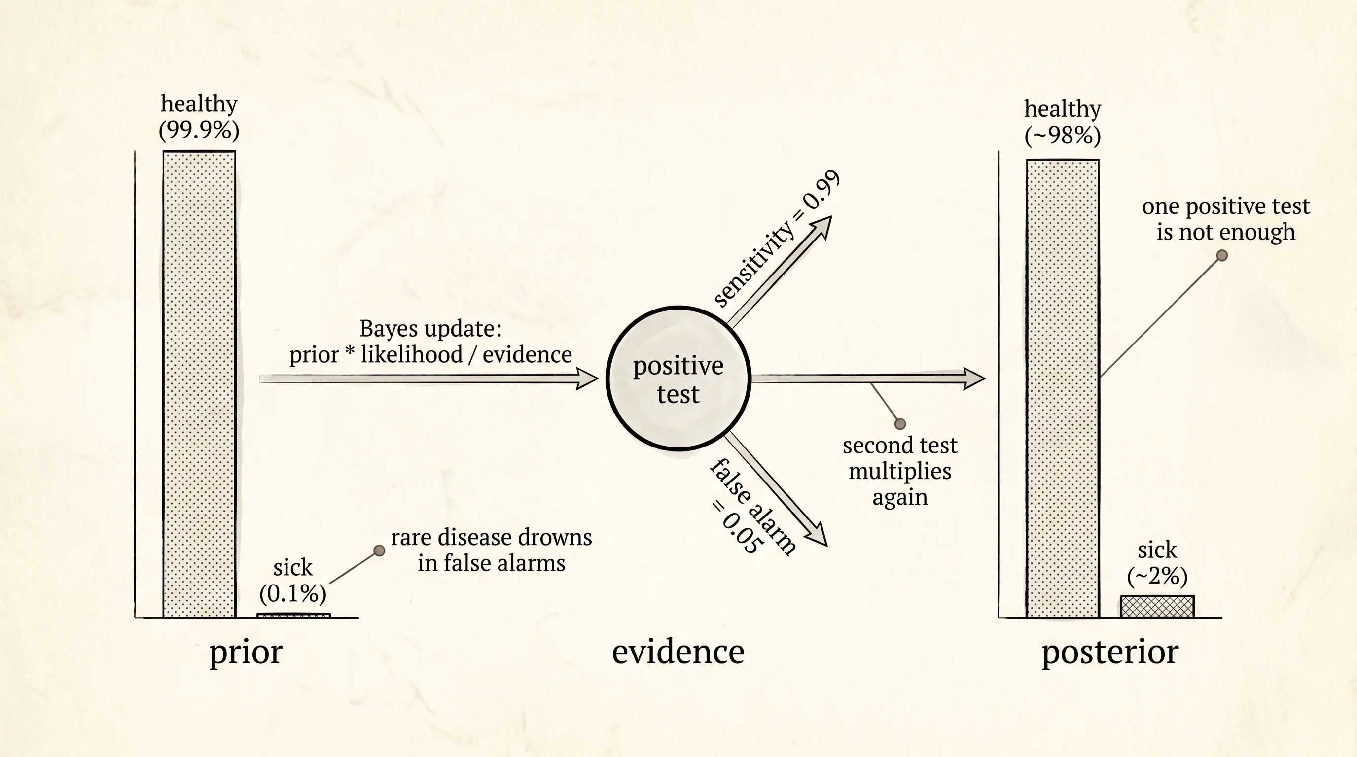
The classic example is a medical test. Suppose a disease shows up in 1 person out of 1,000. There is a test for it that catches the disease 99% of the time when it is there (sensitivity = 0.99) and gives a false alarm 5% of the time when it is not (specificity = 0.95). You take the test. It comes back positive. What is the chance you actually have the disease?
Most people answer 99%. The right answer is closer to 2%.
Do not take that on faith. Simulate it.
def bayes_simulate(prior, sensitivity, specificity, n_trials):
    true_positives = 0
    positive_tests = 0
    for _ in range(n_trials):
        has_disease = random.random() < prior
        if has_disease:
            tested_positive = random.random() < sensitivity
        else:
            tested_positive = random.random() < (1 - specificity)
        if tested_positive:
            positive_tests += 1
            if has_disease:
                true_positives += 1
    if positive_tests == 0:
        return 0.0
    return true_positives / positive_tests


p = bayes_simulate(prior=0.001, sensitivity=0.99, specificity=0.95, n_trials=1_000_000)
print(f"P(disease | positive test) = {p:.4f}")
P(disease | positive test) = 0.0193About 2%. Out of every 100 positive results, only two of those people actually have the disease. The other 98 are false alarms. The reason is the prior — only 1 in 1,000 people has the disease in the first place, so even a small false-positive rate of 5% drowns the true positives in noise. The formula written down later by Bayes and Laplace is
P(disease | positive) = P(positive | disease) * P(disease) / P(positive)
                      = (0.99 * 0.001) / (0.99 * 0.001 + 0.05 * 0.999)
                      ≈ 0.0194
Match. You did not need it. The simulation gave you the answer. The formula explains why the answer is what it is. This is the move every applied probabilist makes, and it is the move every neural network makes when it computes a loss: count what happens, then read off the rule.
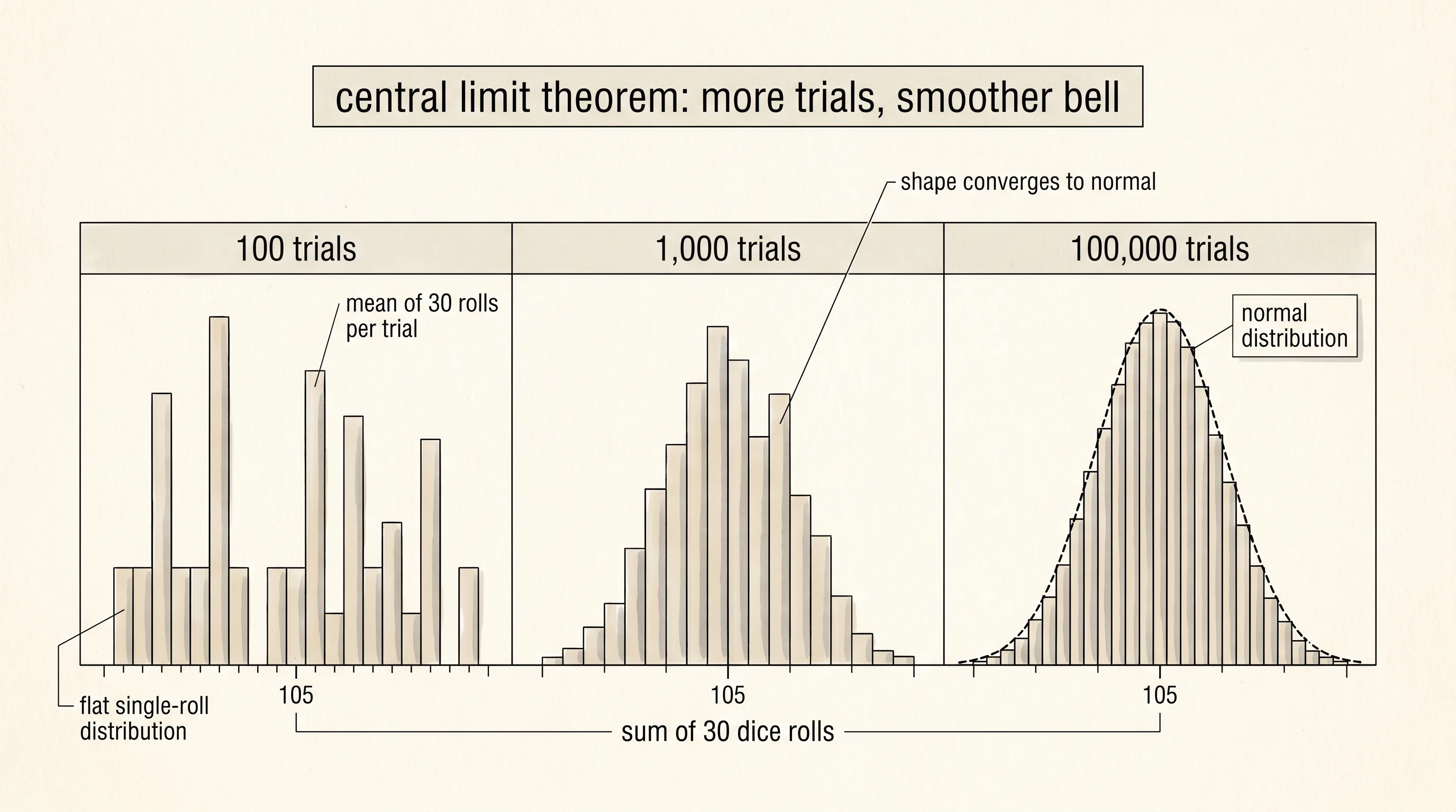
The last big idea is the central limit theorem. Roll the die. The distribution of single rolls is flat — every face equally likely. Now do something different: roll the die 30 times, average those 30 rolls into one number, and call that one number a "sample mean." Repeat that whole experiment ten thousand times. Plot a histogram of the sample means. The distribution of those means is not flat. It is a smooth bell curve centered on 3.5.
def sample_mean(sampler, sample_size):
    return sum(sampler.sample() for _ in range(sample_size)) / sample_size


def clt_demonstrate(sampler, sample_size, n_means):
    return [sample_mean(sampler, sample_size) for _ in range(n_means)]


def ascii_histogram(values, bins=20, height=10):
    lo, hi = min(values), max(values)
    width = (hi - lo) / bins
    counts = [0] * bins
    for v in values:
        idx = min(int((v - lo) / width), bins - 1)
        counts[idx] += 1
    peak = max(counts)
    for row in range(height, 0, -1):
        line = ""
        for c in counts:
            line += "#" if c >= peak * row / height else " "
        print(line)
    print("-" * bins)


means = clt_demonstrate(Die(), sample_size=30, n_means=10000)
ascii_histogram(means)
##
#####
#######
#########
#########
###########
#############
###############
#################
##################
--------------------A bell. The single-roll histogram would be flat. The mean-of-30 histogram is normal, centered on 3.5, narrow. Now switch the sampler. Use a wildly skewed distribution — something that looks nothing like a die — and run the same code:
class Skewed:
    def sample(self):
        # heavy left tail, sharp right cliff
        x = random.random()
        return x ** 4


means = clt_demonstrate(Skewed(), sample_size=30, n_means=10000)
ascii_histogram(means)
You get a bell again. The shape of the mean does not depend on the shape of the source. This is the central limit theorem, proved in the 1920s but anticipated by Laplace a century earlier. It is why the normal distribution shows up everywhere in nature and in deep learning — anything that is a sum or average of many small independent pieces ends up looking normal. Weight initialization in a network, the noise on a gradient, the distribution of activations in a deep stack — all of them lean on this fact.
The thread that runs through everything you just did is the same one Kolmogorov axiomatized: probability is a number between 0 and 1 that you can either compute by counting equally likely outcomes (Cardano), update when new evidence arrives (Bayes), or measure by running the experiment a million times (every simulation in this lesson). When a neural network minimizes cross-entropy, it is finding the parameters that make the observed labels as likely as possible under the model. That is maximum likelihood. The loss is just the negative log of a probability. Probability is not a side topic. It is the criterion the whole field optimizes.
You can compute on numbers, on rates of change, and on uncertainty. You still do not have a structure that holds them all together.