The Kitchen Scale and the Jeweler's Scale
Two scales sit on the kitchen counter. The first is a $20 digital kitchen scale that reads in grams up to 5 kilograms. The second is a jeweler's scale in a glass case that reads down to a thousandth of a gram. Bread dough goes on the kitchen scale. A single grain of saffron goes on the jeweler's. Use the wrong one and the bread dough crashes the jeweler's display, or the grain of saffron reads as zero on the kitchen scale and the recipe loses the most expensive ingredient. Mixed-precision training is the same kitchen. The kitchen scale is fp16, the format that holds a number in 2 bytes. The jeweler's scale is fp32, the format that holds a number in 4. Almost every measurement a neural network needs is bread-dough sized — a forward activation, a typical weight, a typical gradient — and the kitchen scale handles it twice as fast at half the memory. The few measurements that are saffron-sized — the gradients at the bottom of a deep network, the running sum of a loss — still need the jeweler.
The format itself was nailed down in 1985. A committee at the IEEE published standard 754 that year, which fixed exactly how a computer should store a fraction in 32 bits: 1 bit for the sign, 8 for the exponent, 23 for the mantissa. Every scientific calculator, every game, every spreadsheet runs on those 32 bits. Half precision was a side-show until 2017, when NVIDIA shipped the V100 GPU with a new circuit called the tensor core. The tensor core multiplied two 4-by-4 fp16 matrices in a single clock tick — eight times faster than the same multiply at fp32 — but only if the operands were already in fp16. The hardware was ready. The math was not. Nobody had proven you could train a deep network in fp16 without it diverging. In 2018 a team at NVIDIA, lead author Paulius Micikevicius, published Mixed Precision Training and pinned down the recipe: do most of the math in fp16 to feed the tensor cores, keep a master copy of the weights in fp32 so updates do not get rounded away, and multiply the loss by a constant before backprop so the gradients land inside fp16's range. Two years later Google's TPU team shipped bfloat16 — same 16 bits but with fp32's exponent range, no scaling needed — and in 2024 fp8 training started shipping for further throughput. The trend is the same direction every year: fewer bits, more arithmetic per second, the same final model.
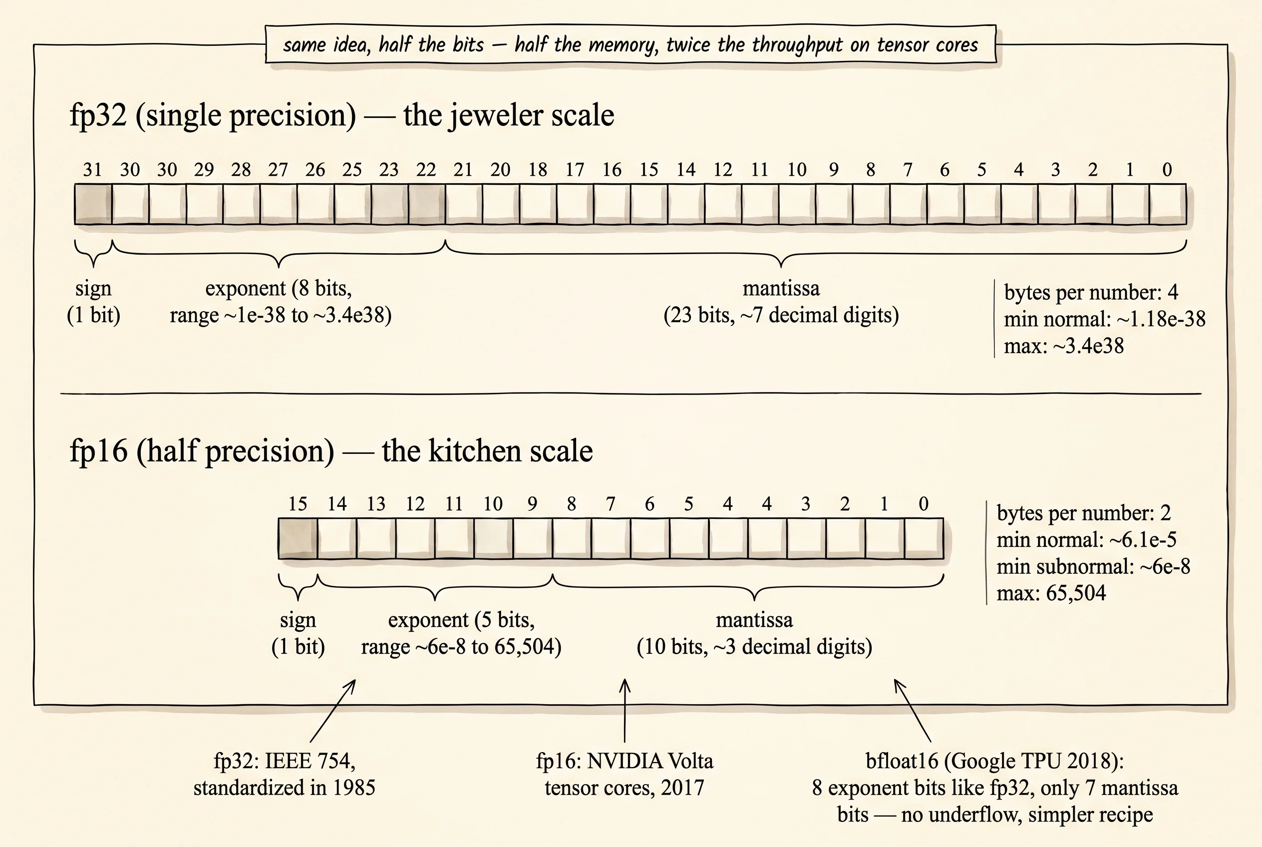
The picture above is the only picture you need for the format. fp32 has 8 bits of exponent and 23 bits of mantissa. The exponent decides how big or small a number can be. The mantissa decides how many digits of resolution it has at that scale. fp16 has 5 bits of exponent and 10 bits of mantissa. Five bits of exponent only reach from about 6 times 10 to the negative 8 on the small end up to 65,504 on the big end. Anything larger than 65,504 becomes positive infinity. Anything smaller than 6 times 10 to the negative 8 becomes zero. Ten bits of mantissa give about 3 decimal digits of resolution. The number 1.0001 is past the grid in fp16 — the closest representable neighbor of 1.0 is something like 1.00098, three digits in, so 1.0001 rounds back to 1.0. Read those three sentences twice. They are the whole tax mixed precision pays.
Open main.py. The plan is to build two classes that simulate the formats on top of Python's native fp64 float, then watch what they do. A real fp16 register would clamp anything bigger than 65,504 to infinity, anything smaller in magnitude than 2 to the negative 24 to zero, and snap the mantissa to 10 bits. A Python float will not do any of that on its own — it has the full 53-bit precision of fp64 — so the simulator does the clamping and rounding by hand on every assignment.
import math

FP16_MAX = 65504.0
FP16_MIN_SUBNORMAL = 2.0**-24
FP16_MANTISSA_BITS = 10


def round_to_mantissa_bits(value: float, mantissa_bits: int) -> float:
    if value == 0.0 or not math.isfinite(value):
        return value
    sign = -1.0 if value < 0.0 else 1.0
    magnitude = abs(value)
    exponent = math.floor(math.log2(magnitude))
    scale = 2.0**exponent
    fraction = magnitude / scale - 1.0
    step = 2.0**-mantissa_bits
    snapped_fraction = round(fraction / step) * step
    return sign * (1.0 + snapped_fraction) * scale
The function decomposes a number the way IEEE 754 does — sign times one-plus-fraction times two-to-the-exponent — and then snaps the fraction to its nearest multiple of 1 / 2^mantissa_bits. Ten bits of mantissa means the step is 1 / 1024. Every fp16 value lives at one of those grid points. Anything between two grid points rounds to the nearest one. The Float16 class wraps the rounding behind a normal-looking number.
class Float16:
    __slots__ = ("value",)

    def __init__(self, value: float) -> None:
        self.value = self._clamp_and_round(float(value))

    @staticmethod
    def _clamp_and_round(value: float) -> float:
        if math.isnan(value):
            return float("nan")
        if value > FP16_MAX:
            return float("inf")
        if value < -FP16_MAX:
            return float("-inf")
        if value == 0.0:
            return 0.0
        if abs(value) < FP16_MIN_SUBNORMAL:
            return 0.0
        return round_to_mantissa_bits(value, FP16_MANTISSA_BITS)
Run the precision sweep. Five values that look almost identical to a human eye land on three different grid points in fp16.
for raw in [1.0, 1.0001, 1.001, 1.01, 1.1]:
    print(f"  {raw:>8} -> fp16: {Float16(raw).value:.10f}")
1.0 -> fp16: 1.0000000000
1.0001 -> fp16: 1.0000000000
1.001 -> fp16: 1.0009765625
1.01 -> fp16: 1.0097656250
1.1 -> fp16: 1.0996093750The number 1.0001 collapses onto 1.0 because the next grid point above 1.0 is 1.0009765625, and 1.0001 is closer to 1.0 than it is to that. The kitchen scale only reads to the gram. A milligram of flour does not move the needle. The number 1.001 lands on 1.0009765625, the first available grid point past 1.0. Every fp16 value between 1.0 and 2.0 lives on that grid of 1024 evenly spaced steps. That is the whole resolution the format gives you in this range.
The next demo is the upper bound. Numbers bigger than 65,504 do not just round — they leave the format entirely and become infinity.
for raw in [1.0, 1000.0, 65504.0, 65505.0, 100000.0]:
    fp16_value = Float16(raw).value
    overflowed = "yes" if math.isinf(fp16_value) else "no"
    print(f"  {raw:>10} -> fp16: {fp16_value:>10}  overflow: {overflowed}")
1.0 -> fp16: 1.0 overflow: no
1000.0 -> fp16: 1000.0 overflow: no
65504.0 -> fp16: 65504.0 overflow: no
65505.0 -> fp16: inf overflow: yes
100000.0 -> fp16: inf overflow: yesA model that is healthy in fp32 can suddenly crash in fp16 the moment one of its activations climbs above 65,504. Once a single number in the network goes to infinity, the multiplications that follow turn the rest of the network's numbers into infinity too, and the loss reads as nan on the next backward pass. That is the failure mode you will read about in every fp16 training log on the internet.
The lower bound is the more interesting one. The diagnostics you built in the gradient-telescope lesson printed the gradient at layer 1 of a depth-50 network as 2.5 times 10 to the negative 18. That number does not exist in fp16. It rounds to zero before the optimizer ever sees it. The sub-analogy here is exactly the diagnostics from the previous lesson — every time you weigh the network's gradient, the kitchen scale either reads a usable number or it reads zero. Watching the scale tell you zero is how you find out the format is the bottleneck.
for raw in [1.0e-3, 1.0e-5, 1.0e-7, 6.0e-8, 1.0e-8, 1.0e-15]:
    fp16_value = Float16(raw).value
    underflowed = "yes" if fp16_value == 0.0 else "no"
    print(f"  {raw:>10.2e} -> fp16: {fp16_value:>10.2e}  underflow: {underflowed}")
1.00e-03 -> fp16: 1.00e-03 underflow: no
1.00e-05 -> fp16: 1.00e-05 underflow: no
1.00e-07 -> fp16: 1.00e-07 underflow: no
6.00e-08 -> fp16: 6.00e-08 underflow: no
1.00e-08 -> fp16: 0.00e+00 underflow: yes
1.00e-15 -> fp16: 0.00e+00 underflow: yesThe cliff is at about 6 times 10 to the negative 8. Above the cliff, the gradient survives the trip into fp16. Below it, the gradient is zero, and the optimizer multiplies zero by the learning rate and updates the weight by zero. The weight never moves. The layer never learns. The whole network silently freezes the first time one of its gradients steps off the cliff.
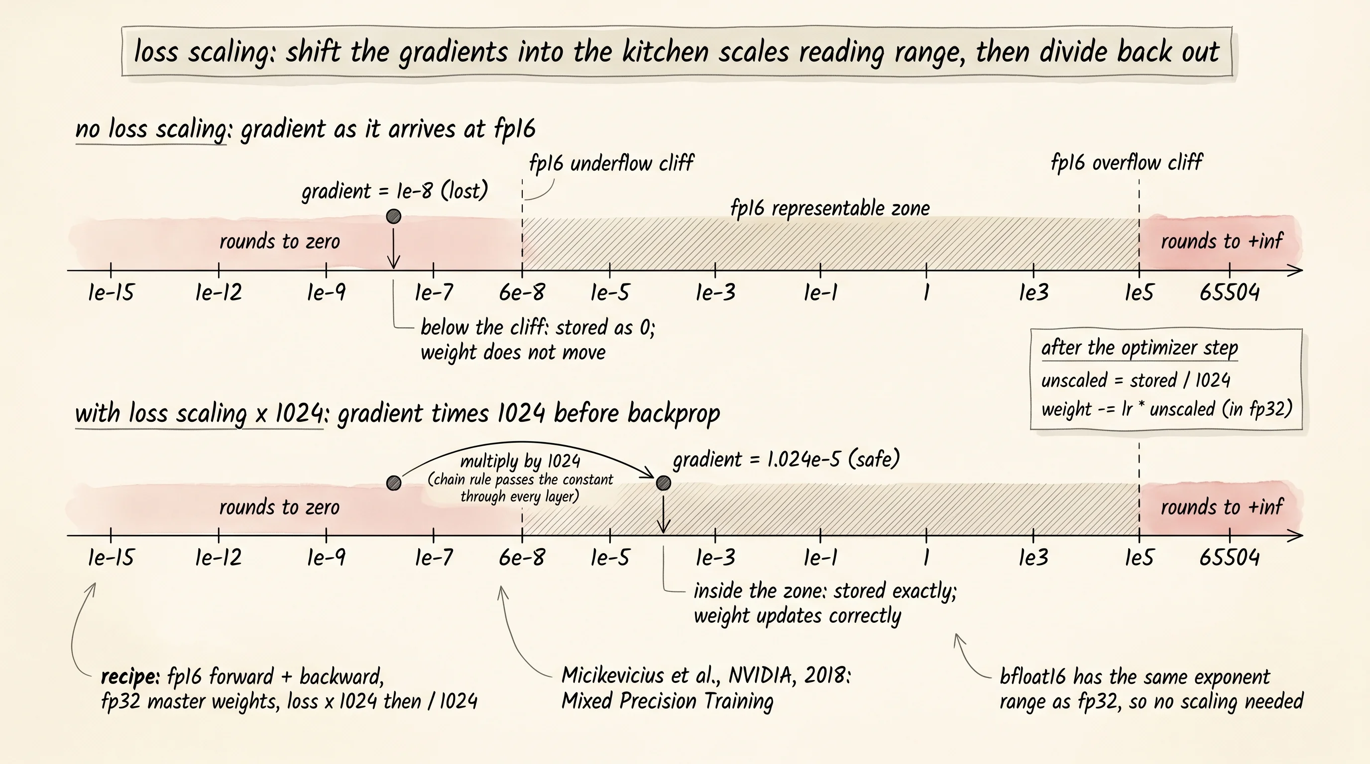
The fix the NVIDIA paper proposed in 2018 was the loss-scaling trick. Multiply the loss by a constant — 1024 is the common choice — before running the backward pass. The chain rule says every gradient in the backward pass picks up the same constant as a multiplier. A gradient of 1 times 10 to the negative 8 — under the cliff — becomes 1.024 times 10 to the negative 5 — well above the cliff. The fp16 version of that scaled gradient is no longer zero. The optimizer still wants the unscaled gradient, so divide by the same constant before the weight update. The math is unchanged. The number that gets stored in fp16 mid-flight is what shifted.
Build the smallest training example that shows the rescue. One linear neuron is learning the rule y = 0.5 * x from twelve random points. The thing that makes this hard for fp16 is the depth-stand-in: every backward pass multiplies the raw gradient by 1e-4, the same way a chain of layers between the loss and this weight would shrink it. Train the same neuron three ways: fp32 baseline, fp16 with no scaling, and fp16 with loss scaled by 1024. The loop tracks how many steps had a gradient that survived in fp64 but rounded to zero after the fp16 squeeze.
def train_in_format(dataset, epochs, learning_rate, use_fp16,
                    chain_shrinkage, loss_scale):
    weight = 0.0
    underflow_steps = 0
    for epoch in range(epochs):
        for x, y in dataset:
            scaled_loss = (weight * x - y) ** 2 * loss_scale
            raw_gradient = 2.0 * (weight * x - y) * x * loss_scale
            shrunk_gradient = raw_gradient * chain_shrinkage
            stored_gradient = (
                Float16(shrunk_gradient).value if use_fp16
                else Float32(shrunk_gradient).value
            )
            if shrunk_gradient != 0.0 and stored_gradient == 0.0:
                underflow_steps += 1
            unscaled_gradient = stored_gradient / loss_scale
            weight -= learning_rate * unscaled_gradient / chain_shrinkage
    return weight, underflow_steps
Look at the order of operations. The loss is scaled up by loss_scale before the gradient is taken. The gradient is shrunk by chain_shrinkage to mimic the depth tax. The shrunk gradient is then squeezed into the chosen format — that is where the underflow check fires. The optimizer divides by loss_scale before applying the step, so the math the network learns from is identical to what fp32 would compute. The only line that changes between the three runs is the format the gradient passes through mid-flight.
Run all three.
  (a) fp32 master weights, no scaling
    final loss 0.0000000000   final weight 0.500000
  (b) fp16 gradients, no scaling
    final loss 0.0000000048   final weight 0.499888
  (c) fp16 gradients, loss scaled by 1024
    final loss 0.0000000000   final weight 0.500000

  underflow steps in (a) fp32:                0
  underflow steps in (b) fp16 no scaling:     87
  underflow steps in (c) fp16 with scaling:   76
Look at (b). The fp16 run with no scaling has 87 steps where the gradient was nonzero in fp64 and zero after the squeeze. Those 87 lost updates push the final weight to 0.499888 instead of 0.500000 — close, but the loss is stuck at a tiny constant because the weight cannot quite reach the target. The kitchen scale read zero on too many measurements and the bread dough never finished proofing. Look at (c). The same fp16 path, but the loss was multiplied by 1024 before the backward pass, so the gradient that reached the format was a thousand times bigger and survived. The final weight is 0.500000, exactly. The final loss matches the fp32 baseline. Half the memory, twice the throughput on a tensor-core GPU, same answer.
A small question. Why does (c) still have 76 underflow steps even though it converged correctly? Because once the network reaches the right answer, the next gradient is genuinely tiny — the loss is near zero, so its derivative is near zero too — and it underflows in fp16. That is harmless. Underflow late in training, after the weight has settled, costs nothing. Underflow early in training, when the weight still needs to move, is what kills the model. Loss scaling does not eliminate underflow. It shifts it from "the early gradients that matter" to "the late gradients that no longer do."
The paper added one more rule that the simulator does not show but the real recipe always uses. The master copy of the weights is held in fp32, not fp16. Forward and backward pass run in fp16 to feed the tensor cores. The optimizer step — weight -= learning_rate * gradient — runs in fp32 against the master copy. The master copy is then cast to fp16 before the next forward pass. The reason is that the update is usually thousands of times smaller than the weight itself, and adding a small fp16 number to a large fp16 number rounds the small number away. The weight never accumulates the tiny improvements. Holding the master in fp32 lets every update land on the weight without rounding. Forward passes pay the kitchen-scale tax. Updates run on the jeweler's. That split is what the word "mixed" in mixed precision means.
The story did not stop at fp16. Google's TPU team had been training in their own format called bfloat16 since 2018 — same 16 bits, but the layout was 1 sign bit, 8 exponent bits, 7 mantissa bits, identical to fp32's exponent range. bfloat16 cannot underflow at the same place fp16 does because its exponent reaches almost as far down as fp32's. Bread-dough resolution dropped from 10 mantissa bits to 7, but every model that needed loss scaling in fp16 trained without it in bfloat16. Hopper GPUs in 2022 added native bfloat16 support and the loss-scaling code started disappearing from training scripts. fp8 training, with two competing layouts called E4M3 and E5M2, is the 2024 frontier. Every two years the format gets smaller and the training recipe gets simpler.
You started this course with an interpreter and a single line of Python. You learned how variables hold names that point at boxes in memory. You learned how loops walk through lists and how functions hide complexity behind a name. You learned how a hash table looks up a value in constant time and how a sort puts a list in order. You learned how a single artificial neuron multiplies its inputs by weights and adds a bias, and how stacking those neurons into a network lets the same idea learn the shape of an image, a sentence, a chess move. You learned how the loss scores the network's mistake, how the gradient says which direction to nudge every weight, how backprop pushes that signal from the loss back to layer 1 by the chain rule. You learned about the diseases that broke deep learning for a decade — vanishing gradients, exploding gradients, dead ReLUs — and the shortcuts that fixed them: better activations, better initializations, residual connections, batch normalization, attention. You learned how a transformer reads a sentence, attends to the words that matter, and emits the next token. You learned how to spread the work across many machines and many GPUs without losing the math. And in this last lesson you learned how to weigh the math itself in fewer bits without losing the answer. That is a brain built from primitives. Every piece is in your hands.
The next page is not a new bottleneck. There is no next bottleneck. There is only a list of three places to go from here, each one a longer path that takes what you built and extends it.