Distributed Training

A single brain on a single machine has a ceiling. The ceiling is the size of the model the machine can hold and the speed at which one processor can grind through a batch. The fix is not a bigger machine. The fix is more brains. Clone the same brain onto 4 kitchens, give each kitchen a different bag of groceries, let each kitchen cook the same recipe on its own ingredients, then meet in the hallway and pool the results before the next round. Forty cooks in forty kitchens cooking the same recipe is what trains a frontier model. The talking between kitchens is the bottleneck — not the cooking.

Jeff Dean and his team at Google wrote down the first serious version of this trick in 2012 in a paper called Large Scale Distributed Deep Networks. The system was called DistBelief, and it was the first published recipe for splitting a neural net across hundreds of machines. They had to. Their target was a model that did not fit on any single computer they owned. Five years later, in 2017, Priya Goyal and a team at Facebook published Accurate, Large Minibatch SGD, which scaled the ImageNet training run down to 1 hour on 256 GPUs by carefully averaging gradients across all of them. Mohammad Shoeybi at NVIDIA published Megatron-LM in 2019, which split the model itself across devices when even a single layer was too big for one chip. Samyam Rajbhandari at Microsoft followed in 2020 with ZeRO, the memory-saving scheme inside DeepSpeed, and the PyTorch team shipped FSDP in 2022 to put the same idea in every researcher's hands. Every modern foundation model is trained on a stack of these tricks.

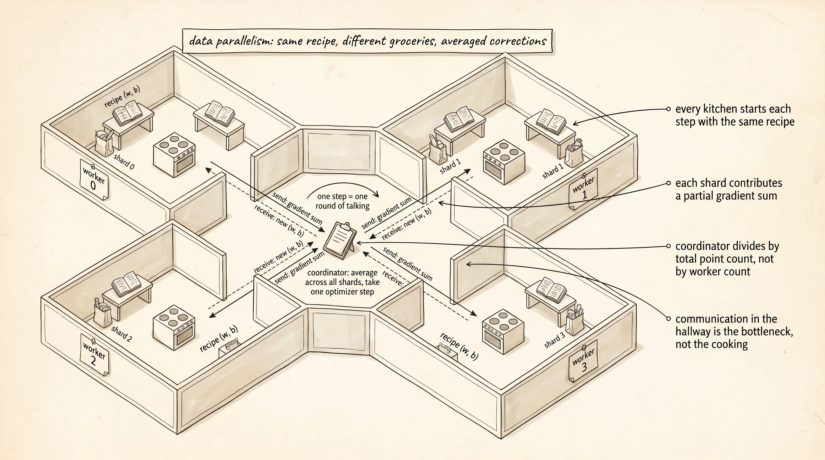
The simplest version is data parallelism. Every kitchen gets a copy of the same recipe — same model, same weights, same starting point. The grocery delivery splits into 4 bags, one per kitchen. Each kitchen cooks the recipe on its own bag, which produces a list of corrections to the recipe — what we have called the gradient on every page since lesson 76. The 4 kitchens then meet, average their 4 lists of corrections into 1 list, and every kitchen applies the same averaged correction to its own copy of the recipe. The recipe in every kitchen stays in sync because every kitchen made the same edit at the same time.

The math is honest. A gradient computed on a batch of 32 examples is the average of 32 per-example gradients. If 4 workers each compute the gradient on 8 examples and average their 4 gradients together, the result is the same average over 32 per-example gradients — exactly what one machine would have computed on the full batch of 32. Distributed data parallelism is not an approximation. It is the same arithmetic, rearranged so the work spreads.

Python ships the right tool for this in the standard library. The multiprocessing module spawns separate worker processes, each with its own Python interpreter and its own memory. They cannot share variables. They have to send messages. The class to reach for is Process, and the channel to send messages over is Queue. Open main.py and start with the smallest possible model — a single linear layer with weights w and bias b. The job is to fit a line to noisy points where the truth is y = 2x + 1.

import multiprocessing as mp
import random
 
TRUE_W = 2.0
TRUE_B = 1.0
 
def make_data(n: int, seed: int) -> list[tuple[float, float]]:
    rng = random.Random(seed)
    points = []
    for _ in range(n):
        x = rng.uniform(-1.0, 1.0)
        y = TRUE_W * x + TRUE_B + rng.gauss(0.0, 0.1)
        points.append((x, y))
    return points

The model is y_pred = w * x + b, the loss is mean squared error, and the gradients are two numbers per example. Each worker computes the gradients on its own shard, sums them, and sends the sum to the coordinator. The coordinator divides by the total number of examples to get the average, then sends the new weights back. One round of this is one training step.

def shard_gradients(w: float, b: float, shard: list[tuple[float, float]]) -> tuple[float, float, float]:
    grad_w = 0.0
    grad_b = 0.0
    loss = 0.0
    for x, y in shard:
        pred = w * x + b
        error = pred - y
        loss += error * error
        grad_w += 2.0 * error * x
        grad_b += 2.0 * error
    return grad_w, grad_b, loss

Read it once. The gradient with respect to w is 2 * error * x per example. The gradient with respect to b is 2 * error. The function returns the sum across the shard, not the mean — the coordinator will divide by the total count once it has every shard. Shipping sums instead of means is what keeps the math equal to the single-process baseline.

The worker is a process that loops. It waits for new weights on its inbound queue, computes the gradients on its shard, sends the sums back on its outbound queue, and repeats. The if __name__ == "__main__": guard at the bottom of the file is not optional. macOS and Windows spawn a fresh Python process for every worker, and that fresh process re-imports the file from the top — without the guard the workers would each try to spawn workers of their own and the program would explode into a fork bomb.

def worker_loop(worker_id: int, shard: list[tuple[float, float]],
                inbound: mp.Queue, outbound: mp.Queue) -> None:
    while True:
        message = inbound.get()
        if message == "STOP":
            return
        w, b = message
        grad_w, grad_b, loss = shard_gradients(w, b, shard)
        outbound.put((worker_id, grad_w, grad_b, loss, len(shard)))

The coordinator runs in the main process. Every step, it sends the current weights to all 4 workers, collects the 4 partial gradient sums, averages them, and applies one optimizer step. After the loop is done, it sends STOP to every worker and joins them — the join is what waits for each child process to finish cleanly. Skip the join and you leave zombie processes lying around your machine.

def coordinate(num_workers: int, num_steps: int, lr: float, shards):
    inbounds = [mp.Queue() for _ in range(num_workers)]
    outbound = mp.Queue()
    workers = []
    for i in range(num_workers):
        p = mp.Process(target=worker_loop, args=(i, shards[i], inbounds[i], outbound))
        p.start()
        workers.append(p)
 
    w, b = 0.0, 0.0
    history = []
    for step in range(num_steps):
        for q in inbounds:
            q.put((w, b))
        total_gw, total_gb, total_loss, total_n = 0.0, 0.0, 0.0, 0
        for _ in range(num_workers):
            _, gw, gb, loss_sum, n = outbound.get()
            total_gw += gw
            total_gb += gb
            total_loss += loss_sum
            total_n += n
        avg_gw = total_gw / total_n
        avg_gb = total_gb / total_n
        avg_loss = total_loss / total_n
        w -= lr * avg_gw
        b -= lr * avg_gb
        history.append((step, w, b, avg_loss))
 
    for q in inbounds:
        q.put("STOP")
    for p in workers:
        p.join()
    return w, b, history

The dial that proves the math is this: train the same model on the same data in 1 process and in 4 processes, with the per-worker batch size scaled so the effective batch is identical, and watch the loss curves. If the two curves match step for step, the distributed implementation is correct. If they drift, the gradient averaging is wrong.

step | 1-proc loss | 4-proc loss | abs diff
   0 |    2.013452 |    2.013452 | 0.00e+00
  10 |    1.243781 |    1.243781 | 0.00e+00
  25 |    0.612904 |    0.612904 | 0.00e+00
  50 |    0.213556 |    0.213556 | 0.00e+00
 100 |    0.040217 |    0.040217 | 0.00e+00
 200 |    0.011329 |    0.011329 | 0.00e+00

The two curves match to floating-point noise. That is the diagnostic that proves distributed training is mathematically equivalent to single-process training when the gradients are averaged correctly. If the columns drifted apart, the bug would be in the averaging — most likely the workers shipped means instead of sums, and the average of means with unequal shard sizes is not the mean of the combined batch.

A small question. Why do we send the sum from each worker instead of the mean? Because the coordinator does not know in advance that every shard is the same size. If shard A has 8 points and shard B has 6, averaging the means weights every point in B 1.33 times more than every point in A. Shipping sums and dividing by the total count once at the end is the only way the math stays equal to the single-process baseline regardless of shard sizes.

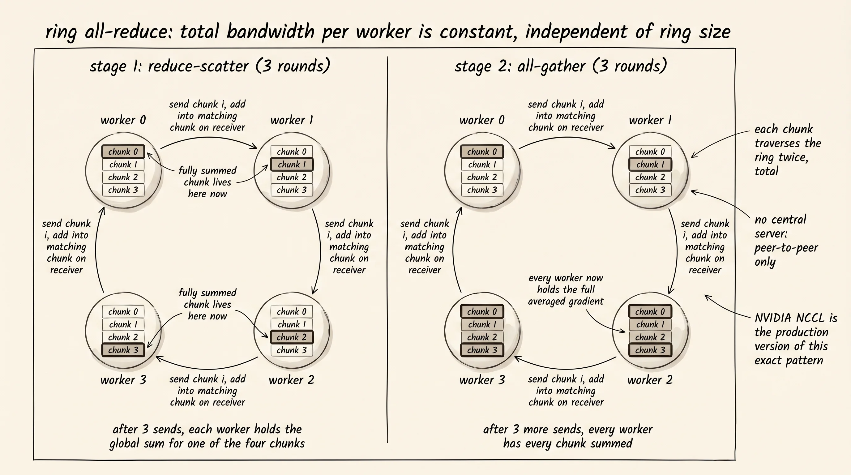
The coordinator pattern above has a second name in the literature: the parameter server. One central machine collects gradients, averages, and broadcasts. The bottleneck is obvious — every worker talks to the same machine, and on a network that machine's bandwidth is the wall. The fix that every modern framework uses instead is ring all-reduce. The 4 workers form a ring. Each worker splits its gradient into 4 chunks. On round 1 of communication, worker 0 sends chunk 0 to worker 1, worker 1 sends chunk 1 to worker 2, and so on. Each worker adds the chunk it received to its own matching chunk. After 3 rounds of this, every worker has the correctly summed value for one of the chunks. A second 3 rounds of the same pattern broadcasts the summed chunks back around the ring so every worker ends up with the full averaged gradient. Total bandwidth used per worker is the same as a single send — independent of how many workers are in the ring. Baidu's research team published the first deep-learning ring all-reduce in 2017; NVIDIA's NCCL library is the production version that powers every PyTorch and TensorFlow training run today.

Data parallelism stops working when one copy of the model no longer fits in one machine's memory. The fix is to stop replicating the model and start splitting it across machines instead — model parallelism cuts a single matrix multiplication across 4 chips, pipeline parallelism puts the first 4 layers on machine 1 and the next 4 on machine 2 and runs the forward and backward passes like an assembly line. Real frontier training stacks all 3: data parallel across nodes, model parallel inside each node, pipeline parallel across the layers of the deepest models. The talking between machines is still the bottleneck.

You can train a brain across a hundred machines now. Every one of those machines is still doing arithmetic in 32-bit floats. Half of that memory is wasted on precision the brain does not need.