Batch Normalization

A brain you build out of layers is alive only as long as signal keeps flowing at a healthy level through every depth. Initialization sets the starting volume. Residual connections give the gradient an express lane. The diagnostics from the last lesson read the brain's vitals layer by layer — the EKG and the bloodwork. The fix that comes after the diagnostics is the brain's circulation system: a small valve at every layer that keeps the blood pressure right no matter what the rest of the body is doing. That valve is batch normalization.

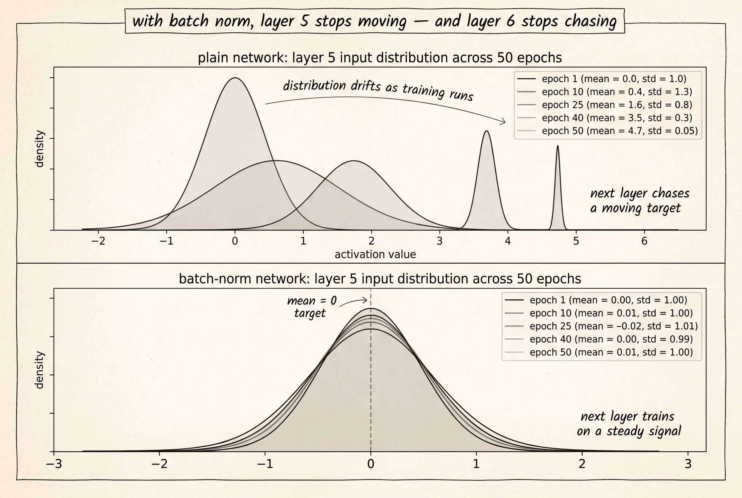
Sergey Ioffe and Christian Szegedy published the paper that named the disease in February 2015. Both worked at Google. They were trying to train deeper Inception networks for image classification and watching the same thing every deep-learning team watched: the longer training ran, the stranger each layer's inputs looked. The output of layer 3 at epoch 1 was a clean Gaussian centered near 0. By epoch 30 the same layer's output had drifted to a mean of 4.7 and a standard deviation of 0.02 — a tight cluster floating far above zero. Layer 4 had spent the first 30 epochs learning weights that worked on Gaussian inputs, and now its inputs were nothing like that anymore. They named the drift internal covariate shift. Their fix was one operation inserted between every layer and the next: take the mini-batch, subtract the batch mean, divide by the batch standard deviation, then scale by a learned number gamma and shift by a learned number beta. The Inception model trained 14 times faster. The paper became one of the most cited machine-learning papers of the decade. A year later Jimmy Ba, Jamie Kiros, and Geoff Hinton at the University of Toronto wrote layer normalization, which does the same arithmetic but across features instead of across the batch — better for recurrent networks where batch size is small or variable. Three years after that, Biao Zhang and Rico Sennrich shipped RMSNorm, the version that drops the mean-subtraction step entirely and that LLaMA and most modern language models use today. Every variant traces back to Ioffe and Szegedy's one observation: the next layer cannot do its job if the input distribution keeps moving.

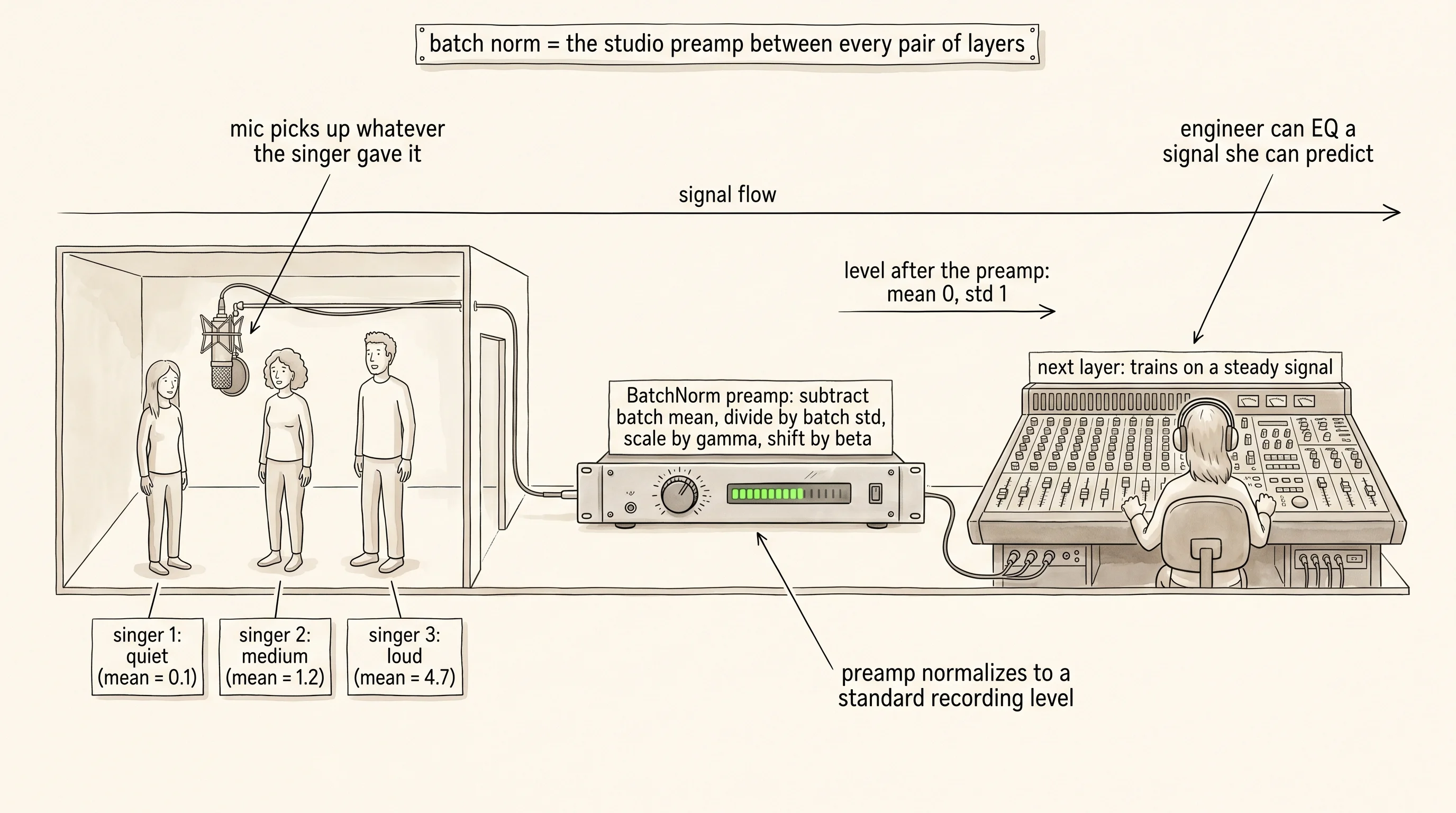
The microphone-gain analogy is the cleanest picture of what is happening. A recording studio puts a singer in front of a microphone and runs the signal through a preamp before it ever reaches the mixing board. The preamp's only job is to level out the volume. A loud singer gets turned down. A quiet singer gets turned up. The output that hits the mixing board is always at a standard recording level no matter who walked into the booth. The mixing engineer, who sits at the next station, gets to apply equalization and compression to a signal she can predict. Without the preamp, the engineer is chasing a moving target — the settings she dialed in for the first singer are wrong for the second, and the recording sounds different on every track. A neural network's hidden layers are the same studio. Layer 4's weights are the engineer's settings. Layer 3's output is the signal arriving from the preamp. If the preamp drifts as training runs, layer 4 is forever rewinding its work to chase the new distribution. Insert a batch-norm layer between every pair of layers and the preamp is back. Layer 4 always sees a signal centered at 0 with standard deviation 1, and its weights stop chasing.

The math is short. A mini-batch is a list of B activation vectors, one per example. Pick one feature dimension. Compute the mean and the variance across the B values in that dimension only. Subtract the mean. Divide by the square root of the variance plus a tiny epsilon to keep the division safe. The result is a list of B values centered at 0 with standard deviation 1. Multiply each by gamma. Add beta. Done. Gamma and beta are two numbers per feature that the network learns alongside the weights. They exist so the network can undo the normalization if it actually wants the layer's input to live somewhere other than mean 0, std 1 — but the optimizer rarely does, because the next layer trains better on a standardized signal. The whole operation, in code, is fewer than ten lines.

import math
 
 
def batch_norm_forward(batch, gamma, beta, epsilon=1e-5):
    batch_size = len(batch)
    feature_count = len(batch[0])
    means = [0.0] * feature_count
    for vector in batch:
        for j in range(feature_count):
            means[j] += vector[j]
    means = [m / batch_size for m in means]
 
    variances = [0.0] * feature_count
    for vector in batch:
        for j in range(feature_count):
            diff = vector[j] - means[j]
            variances[j] += diff * diff
    variances = [v / batch_size for v in variances]
 
    output = []
    for vector in batch:
        normalized = [
            (vector[j] - means[j]) / math.sqrt(variances[j] + epsilon)
            for j in range(feature_count)
        ]
        scaled = [
            gamma[j] * normalized[j] + beta[j]
            for j in range(feature_count)
        ]
        output.append(scaled)
    return output

Read the function. The first block computes the mean of each feature across the batch. The second block computes the variance of each feature across the batch. The third block walks every example, subtracts the mean, divides by the standard deviation, then applies gamma and beta. There is one mean and one variance per feature, not per example. That is the whole reason the operation is called batch normalization — the statistics are taken across the batch dimension.

A worked example pins it down. Imagine a batch of 4 examples, each with 2 features. Three of the examples have the first feature near 0.1 and the fourth has it at 4.7. That is the kind of drift Ioffe and Szegedy saw at layer 5 in epoch 30. Without batch norm, the next layer's weights have to be ready for either kind of input. With batch norm, the four values get re-centered to a mean of 0 and rescaled to a standard deviation of 1 before they ever leave the preamp. The next layer never sees the 4.7. It sees a 1.3 and three small negatives, and it trains on those instead.

batch = [
    [0.10, 0.05],
    [0.08, 0.04],
    [0.12, 0.06],
    [4.70, 0.05],
]
gamma = [1.0, 1.0]
beta = [0.0, 0.0]
 
normalized = batch_norm_forward(batch, gamma, beta)
for vector in normalized:
    print([round(value, 3) for value in vector])

Run it.

[-0.578, -0.555]
[-0.589, -1.665]
[-0.567, 0.555]
[1.734, -0.555]

The first column used to range from 0.08 to 4.70. After the preamp it ranges from -0.59 to 1.73, with a mean of 0 and a standard deviation near 1. The fourth example still stands out — that is the point, the network needs to know that example was different — but it stands out at standard scale, not at scale 50 times larger than its peers. The next layer's weights will not have to chase a moving target.

A small question. What happens to the same operation at inference time, when the network is shown a single example with no batch? You cannot compute a mean and variance from one number. The fix is in project 34: during training, the batch-norm layer also keeps a slow-moving running average of the means and variances it sees. At inference time it uses those running averages instead of the live batch statistics. The forward pass that runs in production does not depend on what other examples happened to be in the batch — and the batch can be size 1.

The diagnostic from the previous lesson is the right place to test this. Project 34 builds two identical 8-layer networks. One has a batch-norm layer between every pair of hidden layers. The other is plain. Both train on the same data, the same number of epochs, the same biased random walk on the weights. The tracker logs the mean and standard deviation of the pre-activation at every hidden layer at every epoch. The print moment is a side-by-side table at epochs 1, 25, and 50. Without batch norm, the standard deviation at layer 1 grows from 0.58 at epoch 1 to 3.58 by epoch 50 — six times its starting value, exactly the kind of drift Ioffe and Szegedy named internal covariate shift. With batch norm, the same number stays near 0.75 the entire run. The same containment shows up at every other hidden layer too. The preamp is doing its job.

That stability is what unlocks the rest of the modern training playbook. Higher learning rates work because the input distribution to every layer is bounded. Initialization choices stop mattering as much because the preamp re-centers whatever the initializer hands it. The internal covariate shift that used to force teams to train shallow networks at low learning rates is gone, and that is why the whole field went deeper after 2015.

One brain on one machine has limits. Real models train on thousands of GPUs at once.