Activation and Gradient Health

The brain you built is a patient. Loss going down is the patient's temperature reading: a single number on a single thermometer that tells you the patient is alive but says nothing about which organ is failing. A real doctor pulls a chart with five rows on it — the EKG for the heart, the bloodwork for the kidneys, the brain scan for the head, the X-ray for the lungs, the reflex test for the nervous system. Each row reads one organ. If the temperature is fine but the EKG is flat, you do not pat the patient on the back and send him home. You stop the visit and figure out why his heart is not beating. A neural network trains the same way. The loss curve is the temperature. The activation distribution at every layer is the EKG, the gradient distribution is the bloodwork, the dead-neuron count is the reflex test, and the saturation rate is the X-ray. You read all five every epoch. If any one of them looks sick before the loss does, you stop and fix it before the patient dies on the table.

Xavier Glorot and Yoshua Bengio at the Université de Montréal wrote the founding paper of this whole field in 2010. Their Understanding the difficulty of training deep feedforward neural networks did the obvious experiment that nobody had bothered to do: train a deep network and, at every epoch, plot the distribution of activations at every layer. The plots told the story instantly. Networks that trained well had activations that stayed Gaussian-shaped from layer 1 to layer L. Networks that failed had layer-1 activations spread wide and layer-10 activations crushed to zero or pinned at saturation. The fix — Xavier initialization — fell out of the diagnostic. You cannot fix what you cannot see, and they were the first to look. Five years later Andrej Karpathy turned the same idea into a teaching practice in his Stanford CS231n class and his blog post A Recipe for Training Neural Networks: print histograms, watch them every epoch, treat any drift as a bug. The modern tooling — TensorBoard at Google in 2015, Weights & Biases as a startup in 2018 — exists to render those histograms in real time so a researcher watching a 12-hour training run can spot a sick layer at hour 1 instead of hour 12.

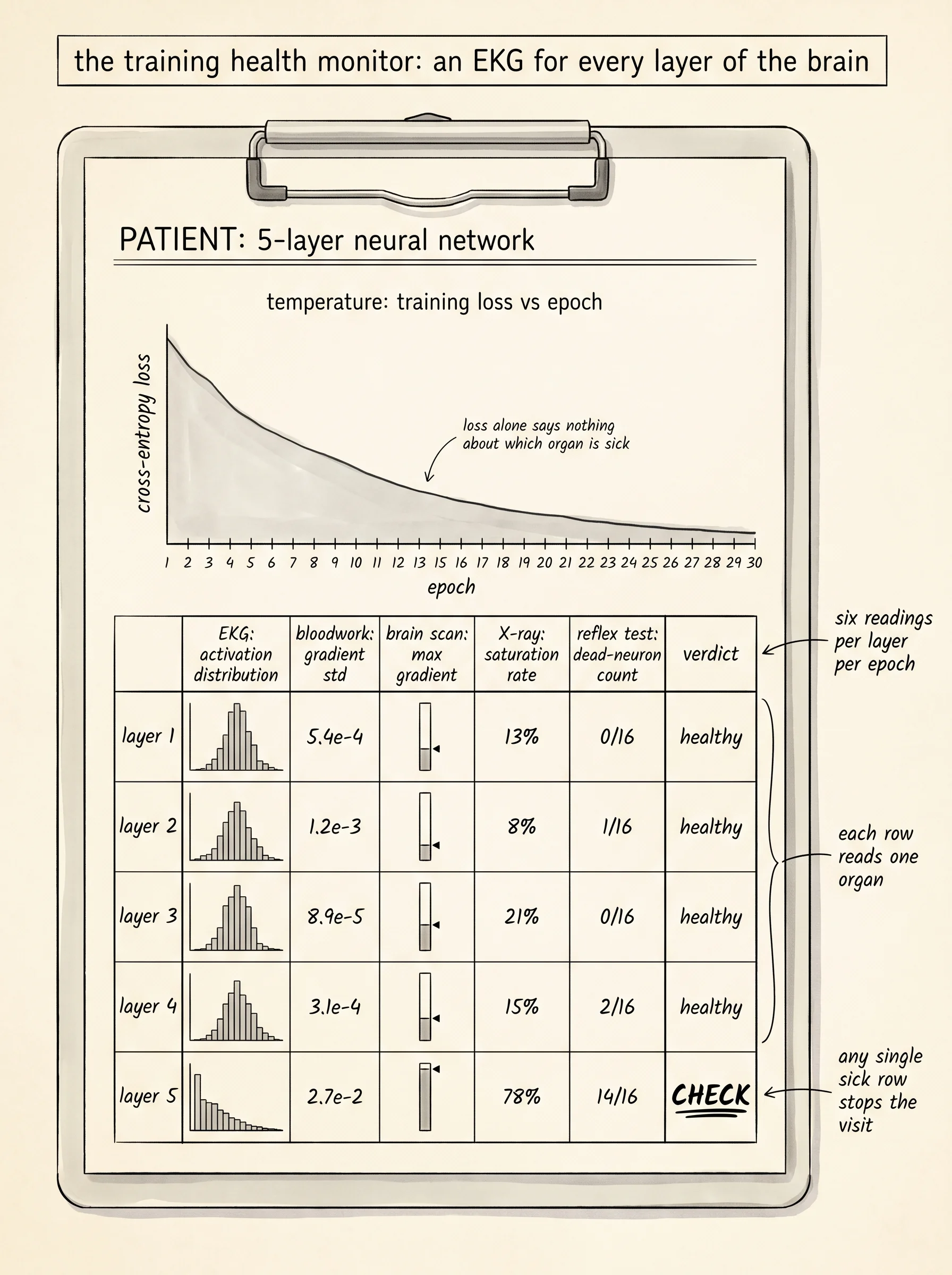
The smallest version of this monitor records six numbers per layer per epoch. Activation mean. Activation standard deviation. Gradient standard deviation. Maximum absolute gradient. Dead-neuron count. Saturation rate. Open main.py in projects/33-training-health-monitor/ and look at the data class.

HealthReport = dict[str, list[float] | list[list[float]] | list[int] | int]

That is the whole shape. One dictionary per epoch. The keys are the names of the readings; the values are lists indexed by layer. The histogram key holds a list of lists — one row per layer, one column per bucket — so the report can also draw a tiny ASCII bar chart of the activation values flowing through every layer. Everything else is a list of plain floats or ints with one entry per hidden layer.

The forward pass needs to write down what it sees, not just the output. Every previous lesson treated the intermediate vectors as throwaway. A diagnostic forward pass keeps them.

def forward_with_trace(network, inputs):
    layer_inputs = []
    pre_activations = []
    post_activations = []
    signal = list(inputs)
    last_index = len(network) - 1
    for layer_index, (weights, biases) in enumerate(network):
        layer_inputs.append(list(signal))
        pre = add_vectors(matvec(weights, signal), biases)
        pre_activations.append(pre)
        if layer_index == last_index:
            post = softmax(pre)
        else:
            post = [safe_relu(value) for value in pre]
        post_activations.append(post)
        signal = post
    return {
        "layer_inputs": layer_inputs,
        "pre_activations": pre_activations,
        "post_activations": post_activations,
    }

The pre-activation is the raw W x + b. The post-activation is what comes out after ReLU. Save both. Mean and standard deviation come from the post-activation. The saturation rate comes from the pre-activation — a pre that has drifted past plus or minus 6 is sitting on the flat shoulder of any reasonable activation function and the gradient through it is dead. The dead-neuron count comes from the post-activation tracked across the whole epoch: the monitor remembers the maximum value every neuron ever produced, and any neuron whose maximum stayed at zero never fired at all.

class TrainingMonitor:
    def __init__(self, layer_widths):
        self.num_hidden_layers = len(layer_widths) - 2
        self.layer_widths = layer_widths
        self.reset()
 
    def record(self, trace, pre_activation_grads):
        for layer_index in range(self.num_hidden_layers):
            pre = trace["pre_activations"][layer_index]
            post = trace["post_activations"][layer_index]
            grad_pre = pre_activation_grads[layer_index]
            self.pre_activations_per_layer[layer_index].extend(pre)
            self.post_activations_per_layer[layer_index].extend(post)
            self.grad_pre_per_layer[layer_index].extend(grad_pre)
            for neuron_index, value in enumerate(post):
                if value > self.neuron_max_per_layer[layer_index][neuron_index]:
                    self.neuron_max_per_layer[layer_index][neuron_index] = value

Every forward pass appends. At the end of the epoch the monitor reduces every accumulator to one summary number per layer. That summary is the report.

The flag function turns the report into English. It reads each layer's row and prints a warning whenever a threshold trips. More than 20 percent of a layer's neurons dead is a warning. Gradient standard deviation below 1e-4 is the vanishing gradient from the previous lesson, named in the report. Gradient standard deviation above 10 is the exploding gradient, also named. Saturation rate above 30 percent is the activation curve being pushed onto its flat shoulder, which is the same disease one hop earlier in the chain. Activation standard deviation collapsing below 1e-3 is signal collapse, the layer producing nearly identical outputs for every input.

def flag_issues(report):
    warnings = []
    for layer_index in range(len(report["activation_mean"])):
        layer_label = f"Layer {layer_index + 1}"
        neuron_count = report["layer_neuron_count"][layer_index]
        dead_count = report["dead_count"][layer_index]
        dead_percent = 100.0 * dead_count / neuron_count
        if dead_percent > 20.0:
            warnings.append(
                f"{layer_label}: {dead_percent:.0f}% dead neurons "
                f"({dead_count}/{neuron_count})"
            )
        gradient_std = report["gradient_std"][layer_index]
        if gradient_std < 1e-4:
            warnings.append(f"{layer_label}: gradient std {gradient_std:.2e} (vanishing)")
        elif gradient_std > 10.0:
            warnings.append(f"{layer_label}: gradient std {gradient_std:.2e} (exploding)")
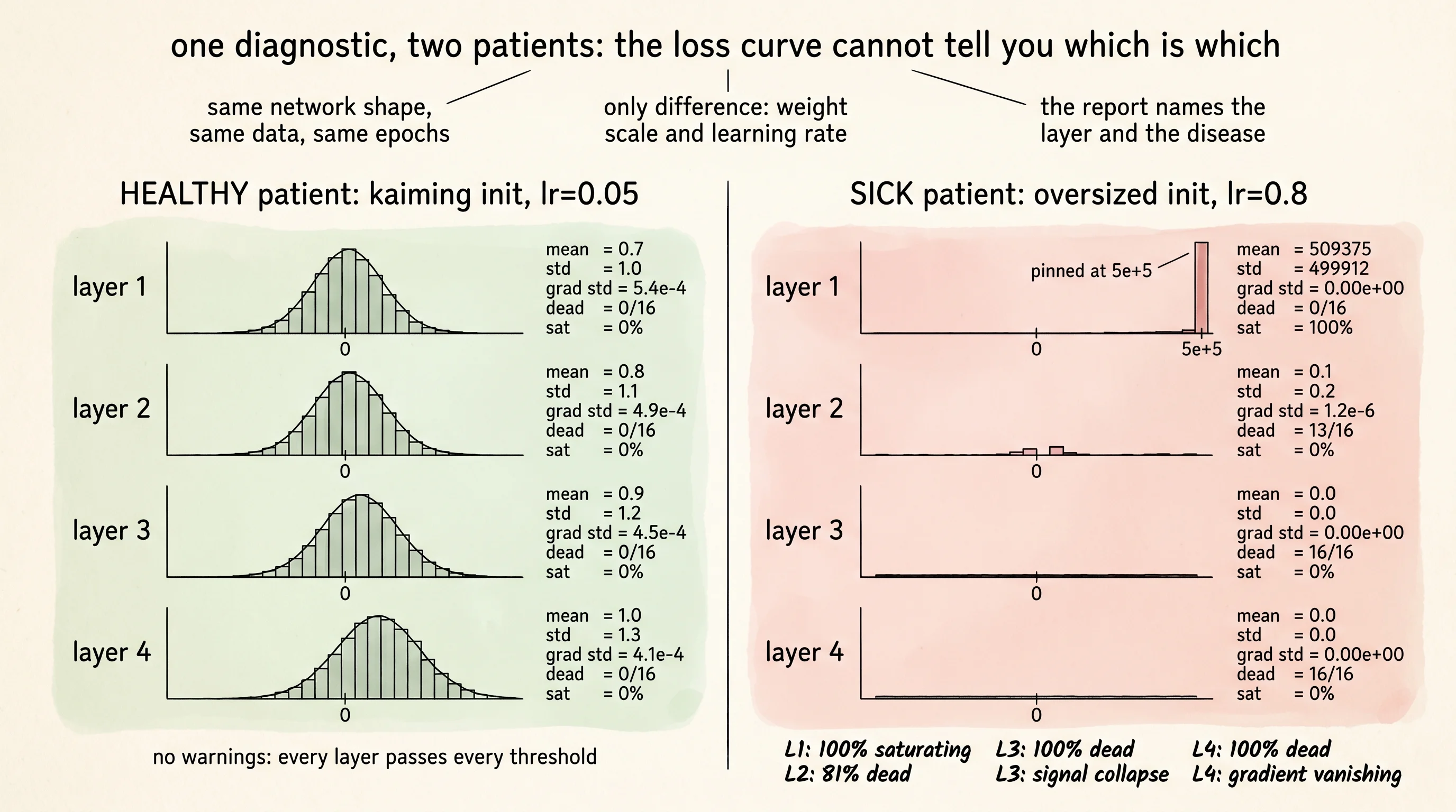
    return warnings

Now train two patients on the same task and run the same diagnostic on both. The healthy patient has Kaiming initialization and a learning rate of 0.05 — the doses every lesson before this one said worked. The sick patient gets an oversized weight scale and a learning rate ten times bigger. Same network shape, same data, same epochs. The only difference is the dosing.

samples = make_training_data(sample_count=80, feature_count=8,
                             class_count=4, seed=7)
 
train(label="HEALTHY (kaiming init, lr=0.05)", layer_widths=[8, 16, 16, 16, 16, 4],
      init_mode="kaiming", weight_scale_override=None, learning_rate=0.05,
      epochs=30, samples=samples, network_seed=11, report_every=10)
 
train(label="SICK (oversized init, lr=0.8)", layer_widths=[8, 16, 16, 16, 16, 4],
      init_mode="bad", weight_scale_override=1.0, learning_rate=0.8,
      epochs=30, samples=samples, network_seed=11, report_every=10)

Run the file. The healthy patient prints first.

=== HEALTHY (kaiming init, lr=0.05) | epoch 30 | per-layer health ===
  layer |  act mean |  act std |  grad std |  max grad |  dead | sat %
  ----- | --------- | -------- | --------- | --------- | ----- | -----
      1 |     0.697 |    1.031 |  5.41e-04 |  8.49e-03 |  0/16 |    0%
      2 |     0.849 |    1.594 |  3.52e-04 |  5.55e-03 |  0/16 |    2%
      3 |     1.258 |    2.208 |  2.73e-04 |  3.99e-03 |  3/16 |    5%
      4 |     2.097 |    3.088 |  2.04e-04 |  2.53e-03 |  2/16 |   13%
  no warnings: every layer is healthy.

Read it row by row. Layer 1's activations have mean 0.7 and standard deviation 1.0 — a clean, wide signal. Layer 4's activations have drifted up to mean 2.1 and standard deviation 3.1, a little wider than ideal because ReLU lets the variance grow on the positive side, but no neuron is fully dead and nothing is saturating. Gradient standard deviation across the four layers ranges from 5e-4 at layer 1 to 2e-4 at layer 4, perfectly within the trainable range. Loss at epoch 30 is 0.0002. The patient is in great shape.

The sick patient prints next.

=== SICK (oversized init, lr=0.8) | epoch 30 | per-layer health ===
  layer |  act mean |  act std |  grad std |  max grad |  dead | sat %
  ----- | --------- | -------- | --------- | --------- | ----- | -----
      1 | 509375.0  | 499912.1 |  0.00e+00 |  0.00e+00 |  0/16 |  100%
      2 |  94037.3  | 290404.1 |  0.00e+00 |  0.00e+00 | 13/16 |  100%
      3 |     0.000 |    0.000 |  0.00e+00 |  0.00e+00 | 16/16 |  100%
      4 |     0.000 |    0.000 |  0.00e+00 |  0.00e+00 | 16/16 |   56%
  WARNINGS:
    - Layer 1: gradient std 0.00e+00 (vanishing)
    - Layer 1: 100% of pre-activations are saturating (|value| > 6)
    - Layer 2: 81% dead neurons (13/16)
    - Layer 3: 100% dead neurons (16/16)
    - Layer 3: activation std 0.00e+00 (signal collapse)
    - Layer 4: 100% dead neurons (16/16)

Layer 1's mean is half a million. Layer 2 is dead in 13 of 16 neurons. Layer 3 and layer 4 are completely silent — every neuron in both layers fires zero across every sample in every batch. The whole back half of the network has flatlined. Gradient standard deviation reads zero everywhere because there is no signal flowing forward, so there is nothing for the loss to differentiate. The cross-entropy loss is 1.59 — barely better than guessing. The sick patient is running on its first two layers only and they are running on saturated, exploded values that learn nothing.

The diagnostic told you all of that without you having to look at a loss curve. That is the entire point. Loss is one number averaged over the whole network; the report is six numbers per layer. The loss curve for the sick run looks suspicious — high and not falling — but it does not tell you which layer is the problem or why. The report names the layer, names the disease, and names the threshold that tripped.

A small question. Why does the sick run show "vanishing gradient" warnings when the disease is exploding pre-activations? Because once a ReLU pre-activation explodes past the safe-relu cap, the post-activation freezes at the cap. Backprop multiplies the upstream gradient by the ReLU derivative, which is 1 for any positive pre-activation, but the upstream gradient itself is the difference between the softmax probabilities and the target one-hot vector. When the softmax sees logits in the millions, one class ends up at probability 1 and the rest at probability 0, so the difference vector is nearly zero for the predicted class and zero for the rest. The exploding forward pass kills the backward pass. The two diseases are the same disease watched from opposite ends. The report catches both because it reads both ends.

This is the lesson where the curriculum stops giving you single fixes and starts giving you instruments. ReLU was a fix. Kaiming initialization was a fix. Residual connections were a fix. The training health monitor is not a fix; it is the medical chart that tells you which fix to reach for. From here on the curriculum is about scale, and at scale you cannot eyeball the problem from a loss curve. A 70-billion-parameter language model has thousands of layers and billions of neurons, and any one of them can be sick while the loss looks fine. The same six readings you just printed for a 5-layer toy network are the same six readings every production training pipeline records every step. The dashboards get fancier; the readings do not change.

The diagnostic told you the sick patient was sick. It did not say what to give him.