What a Neuron Computes
Close the workshop. The four materials are stacked in the corner — numbers, slopes, dice, graphs — and you have everything you need to forge a brain. A brain is not a machine you build all at once. A brain is built out of cells, billions of them, each one a tiny decision-maker. Before you build the brain you build one cell. The cell is called a neuron.
Warren McCulloch and Walter Pitts wrote down the first artificial neuron in 1943. McCulloch was a 44-year-old neurologist at the University of Illinois. Pitts was a 20-year-old runaway who had taught himself logic in a public library in Detroit. They co-wrote a paper called A Logical Calculus of the Ideas Immanent in Nervous Activity and showed that a neuron could be modeled as a switch — it sums up its inputs, and if the sum crosses a threshold, it fires. That was it. No learning, no weights worth tuning, just a logic gate dressed up as biology. Fifteen years later Frank Rosenblatt at Cornell Aeronautical Laboratory took the McCulloch-Pitts neuron and gave it adjustable weights. He called it the perceptron. He built it as physical hardware, the Mark I Perceptron, with 400 photocells wired to motors that turned dials to change the weights. The New York Times in 1958 said the perceptron would soon walk, talk, see, write, reproduce itself, and be conscious of its existence. Then in 1969 two MIT professors, Marvin Minsky and Seymour Papert, published a book called Perceptrons that proved a single-layer perceptron cannot learn the XOR function — a function so simple a child can compute it. Funding for the field collapsed. The first AI winter began. Hold onto that XOR result. The next lesson is about why it killed the field and how one trick brought it back.
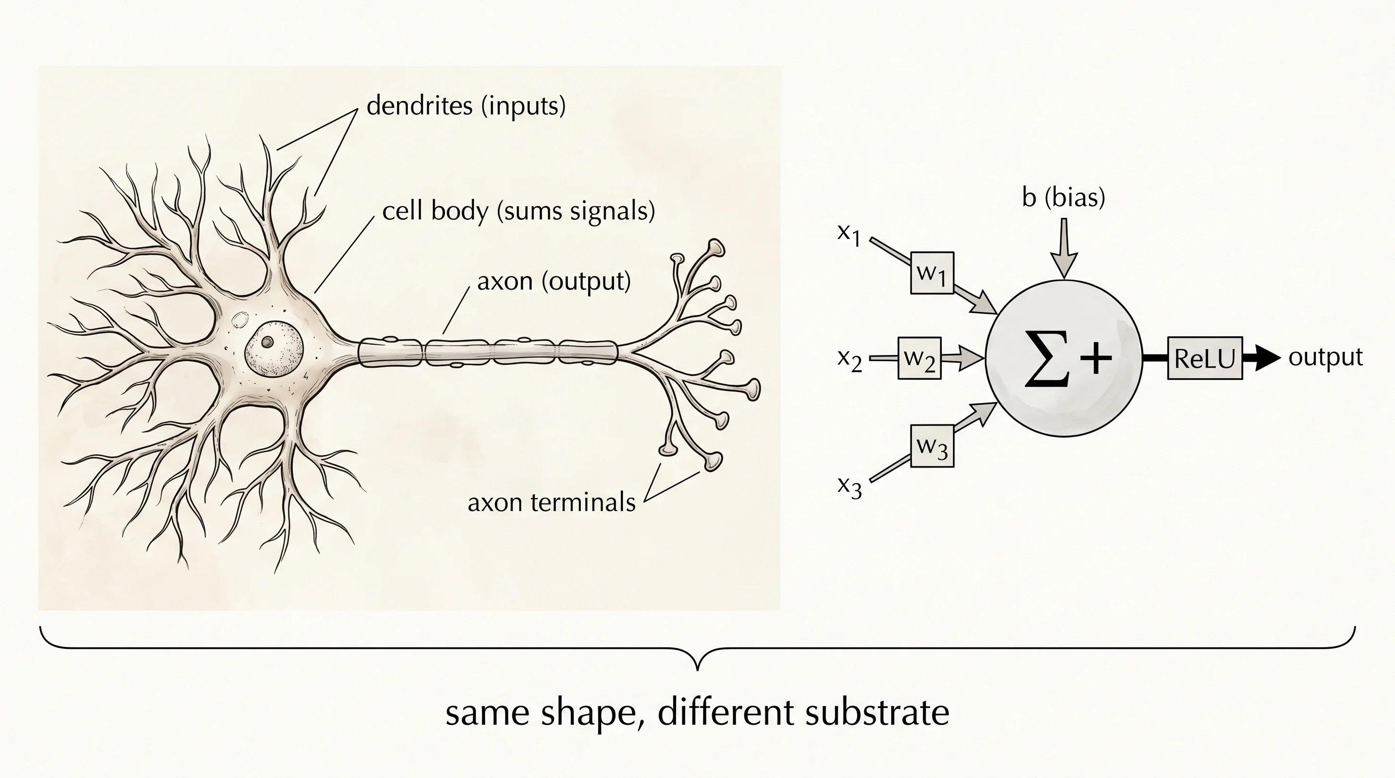
A biological neuron has three parts that matter. Dendrites are the branches that take signals in from other neurons. The cell body adds those signals up. The axon is the single wire that carries the result out to the next neurons. An artificial neuron is a math object with the same shape. It takes a list of input numbers. It multiplies each input by a weight that says how much to trust that input. It adds them all up. It adds one more number called a bias that pushes the total up or down before the decision. Then it passes the total through an activation function — for now, ReLU, which keeps the number if it is positive and replaces it with zero if it is negative. ReLU is the modern stand-in for "the cell fires or stays quiet." That whole operation is one neuron's forward pass. Open neuron.py.
import math
import random


def relu(x):
    return x if x > 0 else 0.0


class Neuron:
    def __init__(self, n_inputs):
        scale = math.sqrt(2.0 / n_inputs)
        self.weights = [random.gauss(0.0, scale) for _ in range(n_inputs)]
        self.bias = 0.0

    def forward(self, inputs):
        total = self.bias
        for w, x in zip(self.weights, inputs):
            total += w * x
        return relu(total)


random.seed(0)
n = Neuron(n_inputs=3)
print("weights:", n.weights)
print("bias:   ", n.bias)
print("output: ", n.forward([1.0, 2.0, 3.0]))
Run it.
weights: [1.4567, -0.2103, 0.9881]
bias:    0.0
output:  3.998
The neuron took three numbers in and gave one number out. The three weights are the three dials on the dendrites. The bias is the fourth dial sitting on the cell body. The output is what travels down the axon. The starting weights came from a Gaussian draw scaled by sqrt(2 / n_inputs) — a recipe Kaiming He published in 2015 to keep the signal from blowing up or dying out as it passes through many layers. Bias starts at zero. None of these numbers were learned yet. The neuron is awake but ignorant.
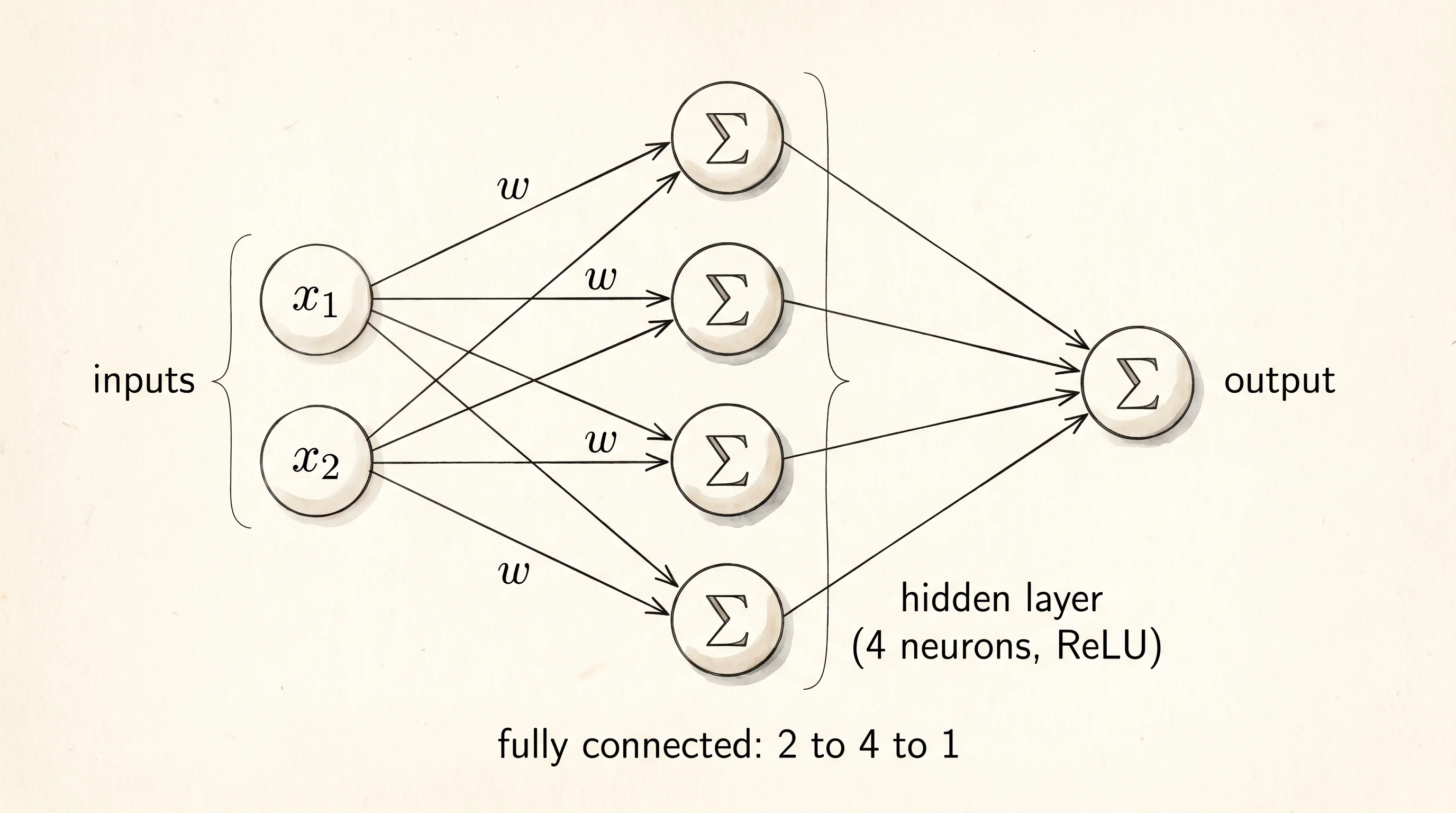
One neuron alone is a single switch. To make a tissue you need a row of them all looking at the same input but each with its own weights, so each neuron learns to detect a different pattern. That row is called a layer. A layer with 8 neurons and 2 inputs has 8 little forward passes happening side by side and produces 8 output numbers. Stack a few layers and the output of one layer becomes the input of the next. That stack is a network.
class Layer:
    def __init__(self, n_inputs, n_neurons):
        self.neurons = [Neuron(n_inputs) for _ in range(n_neurons)]

    def forward(self, inputs):
        return [neuron.forward(inputs) for neuron in self.neurons]


class Network:
    def __init__(self, layers):
        self.layers = layers

    def forward(self, inputs):
        signal = inputs
        for layer in self.layers:
            signal = layer.forward(signal)
        return signal
The Network class is 8 lines and that is most of what every framework on earth does at its core. PyTorch and TensorFlow are mostly bookkeeping around this same forward pass plus a faster way to compute gradients. You will write the faster way in lesson 79. For now, gradients will come from wiggling.
Give the network something to decide. The classic test is: I will throw 2D points at you, some inside a circle and some outside. Tell me which is which. The data is two coordinates, x and y. The label is 1 if the point is inside the circle and 0 if it is outside.
def generate_circle_data(n_points, radius=0.6):
    samples = []
    for _ in range(n_points):
        x = random.uniform(-1.0, 1.0)
        y = random.uniform(-1.0, 1.0)
        label = 1.0 if math.sqrt(x * x + y * y) < radius else 0.0
        samples.append(([x, y], label))
    return samples
A network that is doing well will say close to 1 when you hand it a point inside the circle and close to 0 when the point is outside. A fresh untrained network will say whatever its random weights add up to. The way to teach it: pick a number called the loss that is small when the network is right and big when it is wrong. Squared error works. For each sample, take the network's prediction minus the true label, square it, average over the dataset.
def squared_error(network, data):
    total = 0.0
    for inputs, label in data:
        prediction = network.forward(inputs)[0]
        diff = prediction - label
        total += diff * diff
    return total / len(data)
The loss is one number that scores the whole network. If you wiggle one weight up by a tiny amount, the loss changes by a tiny amount. Divide the change in loss by the change in the weight and you get a slope. The slope tells you which way to nudge that weight to make the loss smaller. Slide the weight in the opposite direction of the slope and the loss drops. Do that for every weight in the network and you have done one step of gradient descent. The slope-by-wiggling trick is called the finite-difference gradient. It is slow because every weight requires two forward passes to measure, but it requires no calculus, no chain rule, no autograd. It just works.
def train(network, data, epochs, lr, eps=1e-3):
    knobs = []
    for layer in network.layers:
        for neuron in layer.neurons:
            for i in range(len(neuron.weights)):
                knobs.append((neuron, "w", i))
            knobs.append((neuron, "b", 0))

    for epoch in range(epochs):
        for neuron, kind, i in knobs:
            current = neuron.weights[i] if kind == "w" else neuron.bias
            if kind == "w":
                neuron.weights[i] = current + eps
            else:
                neuron.bias = current + eps
            loss_high = squared_error(network, data)
            if kind == "w":
                neuron.weights[i] = current - eps
            else:
                neuron.bias = current - eps
            loss_low = squared_error(network, data)
            slope = (loss_high - loss_low) / (2 * eps)
            new_value = current - lr * slope
            if kind == "w":
                neuron.weights[i] = new_value
            else:
                neuron.bias = new_value
        if epoch % 5 == 0:
            print(f"epoch {epoch:>3}: loss = {squared_error(network, data):.4f}")
Before you train, look at what the network thinks. Sample a 20 by 20 grid of points covering the unit square. For each grid point, ask the network for a prediction. If the prediction is 0.5 or higher, mark the cell as "the network says inside." If it is below 0.5, mark it as "the network says outside." Then check what the truth was. The four cases get four characters: # is a correct hit (network said inside, point really is inside), . is a correct miss, o is a false alarm (the network said inside but the point is outside the circle), x is a missed catch (the point is inside but the network said outside).
def render_boundary(network, grid_size=20, radius=0.6):
    rows = []
    for row in range(grid_size):
        cells = []
        for col in range(grid_size):
            x = -1.0 + 2.0 * (col + 0.5) / grid_size
            y = 1.0 - 2.0 * (row + 0.5) / grid_size
            prediction = network.forward([x, y])[0]
            actually_inside = math.sqrt(x * x + y * y) < radius
            predicted_inside = prediction >= 0.5
            if predicted_inside and actually_inside:
                cells.append("#")
            elif predicted_inside and not actually_inside:
                cells.append("o")
            elif not predicted_inside and actually_inside:
                cells.append("x")
            else:
                cells.append(".")
        rows.append(" ".join(cells))
    return "\n".join(rows)
Wire it all up.
random.seed(7)
data = generate_circle_data(200)
network = Network([
    Layer(n_inputs=2, n_neurons=8),
    Layer(n_inputs=8, n_neurons=8),
    Layer(n_inputs=8, n_neurons=1),
])

print("before training:")
print(render_boundary(network))
train(network, data, epochs=120, lr=0.8)
print("after training:")
print(render_boundary(network))
Run it. The before-training grid looks confused. The network's random weights happen to point at one corner of the square, so it thinks half the world is inside the circle and half is outside, but the half it picked has nothing to do with where the circle actually sits.
before training:
. . . . . . . . . . . . o o o o o o o o
. . . . . . . . . . . . . o o o o o o o
. . . . . . . . . . . . . o o o o o o o
. . . . . . . . x x x x . . o o o o o o
. . . . . . x x x x x x x x o o o o o o
. . . . . x x x x x x x x x x o o o o o
. . . . . x x x x x x x x x x . o o o o
. . . . x x x x x x x x x x x x . . . o
. . . . x x x x x x x x x x x x . . . .
. . . . x x x x x x x x x x x x . . . .
The x cells are inside the circle (the network missed them). The o cells outside the circle (the network thought they were inside). Mostly mistakes. Now training runs for 120 epochs of finite-difference gradient descent. It takes about 30 seconds. The loss prints every 5 epochs and drops from 0.35 toward 0.05.
after training:
. . . . . . . . . . . . . . . . . . . .
. . . . . . . . x # # # o . . . . . . .
. . . . . . x # # # # # # # o . . . . .
. . . . . x # # # # # # # # # o . . . .
. . . . . # # # # # # # # # # o o . . .
. . . . x # # # # # # # # # # # o . . .
. . . . # # # # # # # # # # # # . . . .
. . . . # # # # # # # # # # # # . . . .
. . . . # # # # # # # # # # # # . . . .
. . . . . # # # # # # # # # # . . . . .
. . . . . # # # # # # # # # # . . . . .
. . . . . . # # # # # # # # . . . . . .
. . . . . . . . x # # # o . . . . . . .
. . . . . . . . . . . . . . . . . . . .
The dots crowded into the corners. The hashes pooled into a circle in the middle. A handful of o and x cells linger around the edge where the boundary is fuzziest. The network learned where the circle is by nothing but wiggling weights and watching the loss go down. No formula for circles, no rule about distance from the origin, nothing the programmer told it. Each of the 89 weights and 17 biases got tuned 120 times until the right shape emerged.
What happened? Each neuron in the first layer learned to draw a half-plane — a straight line splitting the square into two regions, with one side firing and the other side dark. Eight neurons drew eight half-planes from different angles. The next layer combined those half-planes into more complex regions. The output neuron added them all up into a single yes-or-no number. The reason it can build a curved boundary out of straight cuts is the ReLU between the layers. A pure stack of linear operations cannot do this. Stack 100 layers of weighted sums with no activation in between and the entire thing collapses to one weighted sum — one straight line — no matter how deep you go. The next lesson proves it.