Why Nonlinearity Is Required

Stack neurons all you want — line up a hundred layers, give each one a thousand neurons — and without one trick the whole stack collapses to a single neuron. The trick is nonlinearity. Picture a row of mirrors bouncing a beam of light down a hallway. Each mirror redirects the beam, but the final ray that comes out the far end is still a straight line; the mirrors only ever rotated the direction. Drop a glass prism into the middle of the row and the beam splits into a fan of colors, each one bending differently. The hallway becomes more than the sum of its mirrors. Inside a neural network the activation function is the prism. Without it the layers are mirrors. With it the network can curve.

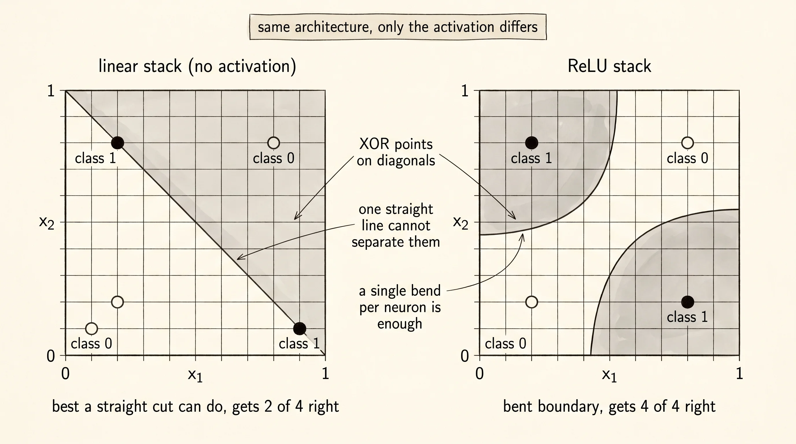
Marvin Minsky and Seymour Papert proved this the hard way in 1969. Both were professors at MIT, and they had grown impatient with Frank Rosenblatt's perceptron — the trainable single-layer network from the previous lesson that the New York Times had promised would soon be conscious. They wrote a book called Perceptrons whose central proof concerned a function so simple a child can compute it: XOR, the exclusive-or. Two binary inputs go in, one binary output comes out. The output is 1 when the inputs disagree (one is 1, the other is 0) and 0 when they agree. Four input pairs total. Try to draw a single straight line through the unit square that puts the two 1-points on one side and the two 0-points on the other side. It cannot be done — the 1-points sit on one diagonal and the 0-points sit on the other. A single-layer perceptron is exactly such a line. Minsky and Papert showed it was, full stop, mathematically incapable of learning XOR. Funding evaporated. The first AI winter began and lasted a decade. Twenty years later George Cybenko at Tufts proved the way out: in a 1989 paper called Approximation by Superpositions of a Sigmoidal Function, he showed that one hidden layer of neurons with a nonlinear activation can approximate any continuous function on a closed bounded region to any precision you want. Two years after that Kurt Hornik in Vienna strengthened the result — the universal approximation property holds for a wide family of activations, not just the sigmoid Cybenko had used. The theorem became known as universal approximation. The hidden layer was the prism.

The way to feel the proof is to build both networks side by side and watch one fail. Pure Python, no libraries — same as the last lesson. A LinearLayer is a row of weighted-sum neurons with no activation at all. A NonlinearLayer is the same row with ReLU clamped on the end. ReLU keeps the number if it is positive and replaces it with zero if it is negative; that single bend is the nonlinearity that does all the work.

import math
import random
 
 
def relu(x):
    return x if x > 0 else 0.0
 
 
class LinearLayer:
    def __init__(self, n_inputs, n_neurons):
        scale = math.sqrt(2.0 / n_inputs)
        self.weights = [
            [random.gauss(0.0, scale) for _ in range(n_inputs)]
            for _ in range(n_neurons)
        ]
        self.biases = [0.0 for _ in range(n_neurons)]
 
    def forward(self, inputs):
        outputs = []
        for row, bias in zip(self.weights, self.biases):
            total = bias
            for w, x in zip(row, inputs):
                total += w * x
            outputs.append(total)
        return outputs
 
 
class NonlinearLayer(LinearLayer):
    def forward(self, inputs):
        return [relu(value) for value in super().forward(inputs)]

The layers store weights as a list of rows so each row is one neuron's weight vector. A Network is a stack of layers exactly like the last lesson, and forward just walks the stack passing the output of one layer into the next.

class Network:
    def __init__(self, layers):
        self.layers = layers
 
    def predict(self, inputs):
        signal = inputs
        for layer in self.layers:
            signal = layer.forward(signal)
        return signal[0]

XOR is four points and four labels. Generate them by hand.

def generate_xor_data():
    return [
        ([0.0, 0.0], 0.0),
        ([0.0, 1.0], 1.0),
        ([1.0, 0.0], 1.0),
        ([1.0, 1.0], 0.0),
    ]

Build two networks of the same shape — 2 inputs, 4 hidden, 4 hidden, 1 output — one all linear and one with ReLU on the hidden layers. Train both with finite-difference gradient descent, the same wiggling routine from dl-neuron. After training, sample a 20 by 20 grid of points and print where each network thinks the answer is 1 (#) versus 0 (.).

random.seed(7)
linear_net = Network([
    LinearLayer(2, 4),
    LinearLayer(4, 4),
    LinearLayer(4, 1),
])
 
random.seed(7)
nonlinear_net = Network([
    NonlinearLayer(2, 4),
    NonlinearLayer(4, 4),
    LinearLayer(4, 1),
])
 
data = generate_xor_data()
train(linear_net, data, epochs=200)
train(nonlinear_net, data, epochs=200)

The training loop is identical — same step size, same epoch count, same starting seed — so the only difference between the two networks is the ReLU. The linear network's loss flatlines at 0.25 after about 20 epochs and refuses to go lower. The nonlinear network's loss rolls down to essentially zero. Print the boundaries side by side.

linear (no activation)                 nonlinear (ReLU)
# # # # # # # # # # # # # # # # # #    # # # # # # # # # # # # # # . . . . . .
# # # # # # # # # # # # # # # # # #    # # # # # # # # # # # # # . . . . . . .
# # # # # # # # # # # # # # # # . .    # # # # # # # # # # # # . . . . . . . .
# # # # # # # # # # # # # # # . . .    # # # # # # # # # # # . . . . . . . . .
# # # # # # # # # # # # # # . . . .    # # # # # # # # # # . . . . . . . . . .
# # # # # # # # # # # # # . . . . .    # # # # # # # # # . . . . . . . . . . #
# # # # # # # # # # # # . . . . . .    # # # # # # # # . . . . . . . . . . # #
# # # # # # # # # # . . . . . . . .    # # # # # # # . . . . . . . . . . # # #
# # # # # # # # # . . . . . . . . .    # # # # # # . . . . . . . . . . # # # #
. . . . . . . . . . . . . . . . . .    # # # # . . . . . . . . . . . . # # # #

The left grid is one straight diagonal cut. That is everything a stack of three linear layers can ever produce. The right grid bends — two of the four corners say 1, the other two say 0, exactly the XOR shape. Same architecture, same data, same gradient descent. Only the prism differs.

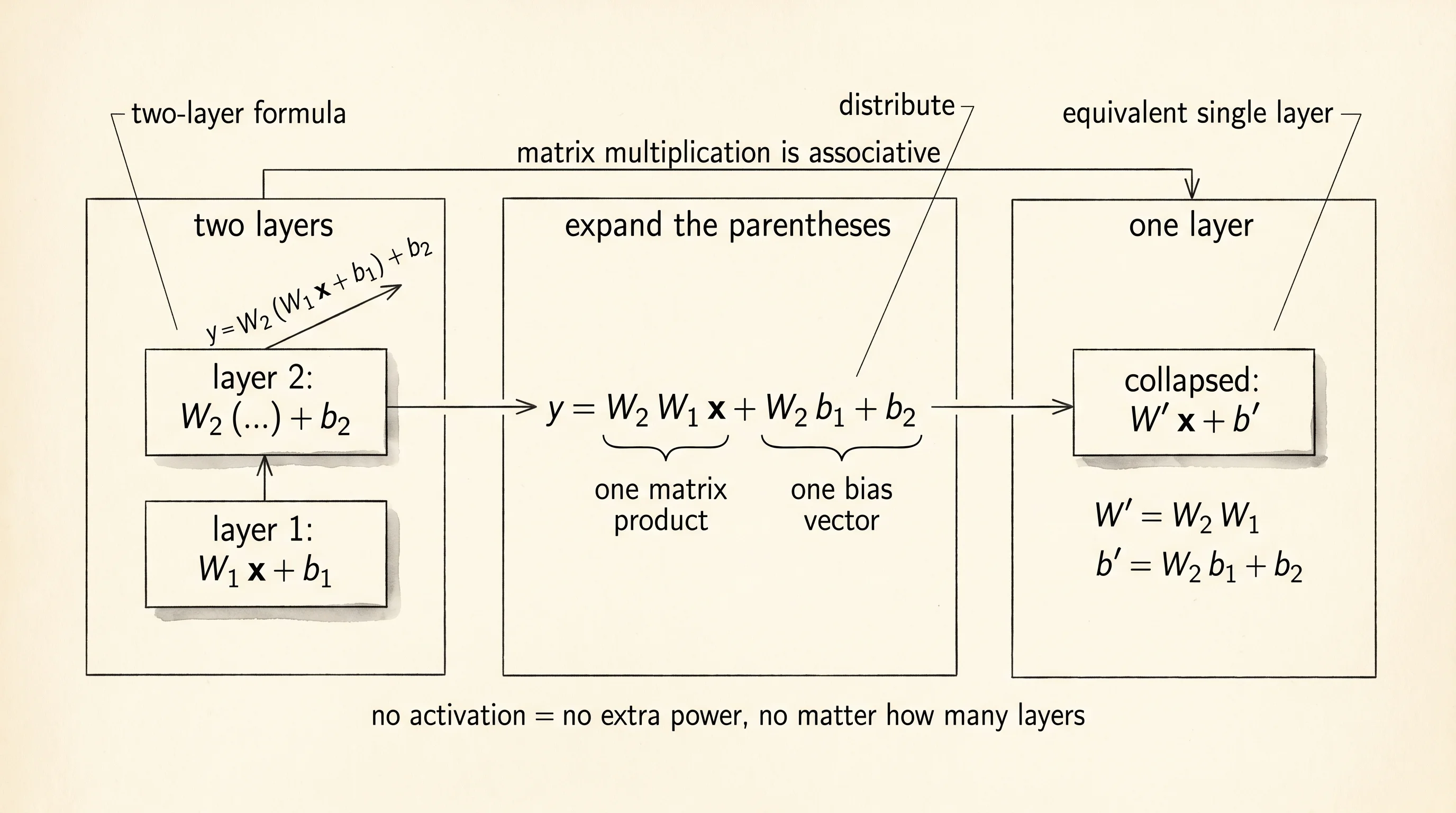
Why does the linear stack fail no matter how deep you make it? Because matrix multiplication is associative. A layer with no activation is output = W x + b. Stack two of them and you get y = W2 (W1 x + b1) + b2. Multiply through and the parentheses dissolve into y = (W2 W1) x + (W2 b1 + b2). The product W2 W1 is one matrix. The vector W2 b1 + b2 is one bias. The two-layer linear network has the exact same expressive power as a single layer whose weights are the product. Stack 100 layers and you get one matrix product times one giant bias — still one straight line in the input space, just a more expensively computed one.

To see this on the page, take a tiny linear stack and multiply its layers by hand. Two layers, both 2-by-2, with numbers small enough to compute mentally.

class TinyLinear:
    def __init__(self, weights, biases):
        self.weights = weights
        self.biases = biases
 
    def forward(self, inputs):
        outputs = []
        for row, bias in zip(self.weights, self.biases):
            total = bias + sum(w * x for w, x in zip(row, inputs))
            outputs.append(total)
        return outputs
 
 
def matmul(a, b):
    return [
        [sum(a[i][k] * b[k][j] for k in range(len(b))) for j in range(len(b[0]))]
        for i in range(len(a))
    ]
 
 
def matvec(a, v):
    return [sum(row[j] * v[j] for j in range(len(v))) for row in a]
 
 
def vec_add(u, v):
    return [a + b for a, b in zip(u, v)]
 
 
layer1 = TinyLinear(
    weights=[[1.0, 2.0], [3.0, 4.0]],
    biases=[1.0, 1.0],
)
layer2 = TinyLinear(
    weights=[[0.5, 0.0], [1.0, -1.0]],
    biases=[2.0, 0.0],
)
 
stacked_output = layer2.forward(layer1.forward([1.0, 1.0]))
 
collapsed_weights = matmul(layer2.weights, layer1.weights)
collapsed_biases = vec_add(matvec(layer2.weights, layer1.biases), layer2.biases)
collapsed = TinyLinear(collapsed_weights, collapsed_biases)
collapsed_output = collapsed.forward([1.0, 1.0])
 
print("layer1 W:", layer1.weights, "b:", layer1.biases)
print("layer2 W:", layer2.weights, "b:", layer2.biases)
print("collapsed W:", collapsed.weights, "b:", collapsed.biases)
print("stacked output:  ", stacked_output)
print("collapsed output:", collapsed_output)

Run it.

layer1 W: [[1.0, 2.0], [3.0, 4.0]] b: [1.0, 1.0]
layer2 W: [[0.5, 0.0], [1.0, -1.0]] b: [2.0, 0.0]
collapsed W: [[0.5, 1.0], [-2.0, -2.0]] b: [2.5, 0.0]
stacked output:   [4.0, -4.0]
collapsed output: [4.0, -4.0]

Verify the collapsed weight matrix by hand. Row 0 of W2 @ W1 is row 0 of W2 (which is [0.5, 0.0]) dotted against each column of W1. Column 0 of W1 is [1, 3], so entry (0,0) is 0.5*1 + 0*3 = 0.5. Column 1 of W1 is [2, 4], so entry (0,1) is 0.5*2 + 0*4 = 1.0. Row 1 of W2 is [1, -1]. Against column 0 of W1: 1*1 + (-1)*3 = -2. Against column 1: 1*2 + (-1)*4 = -2. The product matrix is [[0.5, 1.0], [-2.0, -2.0]] — which is exactly what the program printed. Two layers of math became one.

What was the proof? The stacked output and the collapsed output are the same number, to the bit. They were the same function the entire time. Hide the print statement and no observer downstream of the network could ever tell whether you ran the two layers or the one collapsed layer. Now drop the ReLU back into the middle and try to multiply it out. ReLU is max(0, x). There is no matrix you can pre-compute that captures it, because the operation it performs depends on whether the running total is positive or negative — a decision made at runtime, per neuron, per input. The instant a per-input decision sneaks into the computation, the algebra stops being linear and the layers stop collapsing. The boundary stops being a straight line. Cybenko's theorem becomes available. Hornik's extension follows. Everything that came after — vision models, language models, the whole second wave of AI — required this single trick.

You proved you need a nonlinearity. Now meet the first one anyone tried.