The Sigmoid Curve

Drop a single bacterium into a petri dish and check back every hour. The first few hours are flat. Then the colony doubles, and doubles again, and the curve climbs like a wall. Then the food runs out. The curve bends, slows, and flattens against a ceiling. The shape it traces from start to finish is a long, lazy S. The same S shows up when a new product spreads through a city, when a rumor crosses a school, when a virus moves through a population. The S-curve was a fact about life and money for 100 years before anyone wired it into a neural network. The first nonlinearity that backprop ever used was already on a chalkboard in Belgium in 1838.

Pierre Francois Verhulst was a 34-year-old Belgian mathematician staring at population tables. Thomas Malthus had warned in 1798 that any population grows exponentially and any food supply grows at most linearly, so famine was inevitable. The math was clean but the data refused to cooperate. Real populations slowed down. Verhulst's fix was one extra term. Growth is proportional to the population for now, and proportional to the room left in the world. Pile a thousand more rabbits into the meadow and the next litter is smaller, because there is less grass to go around. Verhulst wrote down a differential equation for that idea and solved it. The solution was the sigmoid. He published it in 1838 and almost nobody read it. The paper sat in a drawer for 82 years. In 1920 Raymond Pearl and Lowell Reed at Johns Hopkins were fitting curves to the United States census and rediscovered the same equation, gave it the name "logistic growth," and put it on a respectable scientific footing. Through the 1940s and 50s it modeled chemical reactions, the spread of telephones, the adoption of hybrid corn in Iowa. Then in the 1980s, when David Rumelhart and Geoffrey Hinton needed a smooth squashing function for backpropagation, they reached for the same curve. It had two things going for them: it pinned its output between 0 and 1, and it was differentiable everywhere. Backprop needs a slope at every point, and the sigmoid hands one over without complaint.

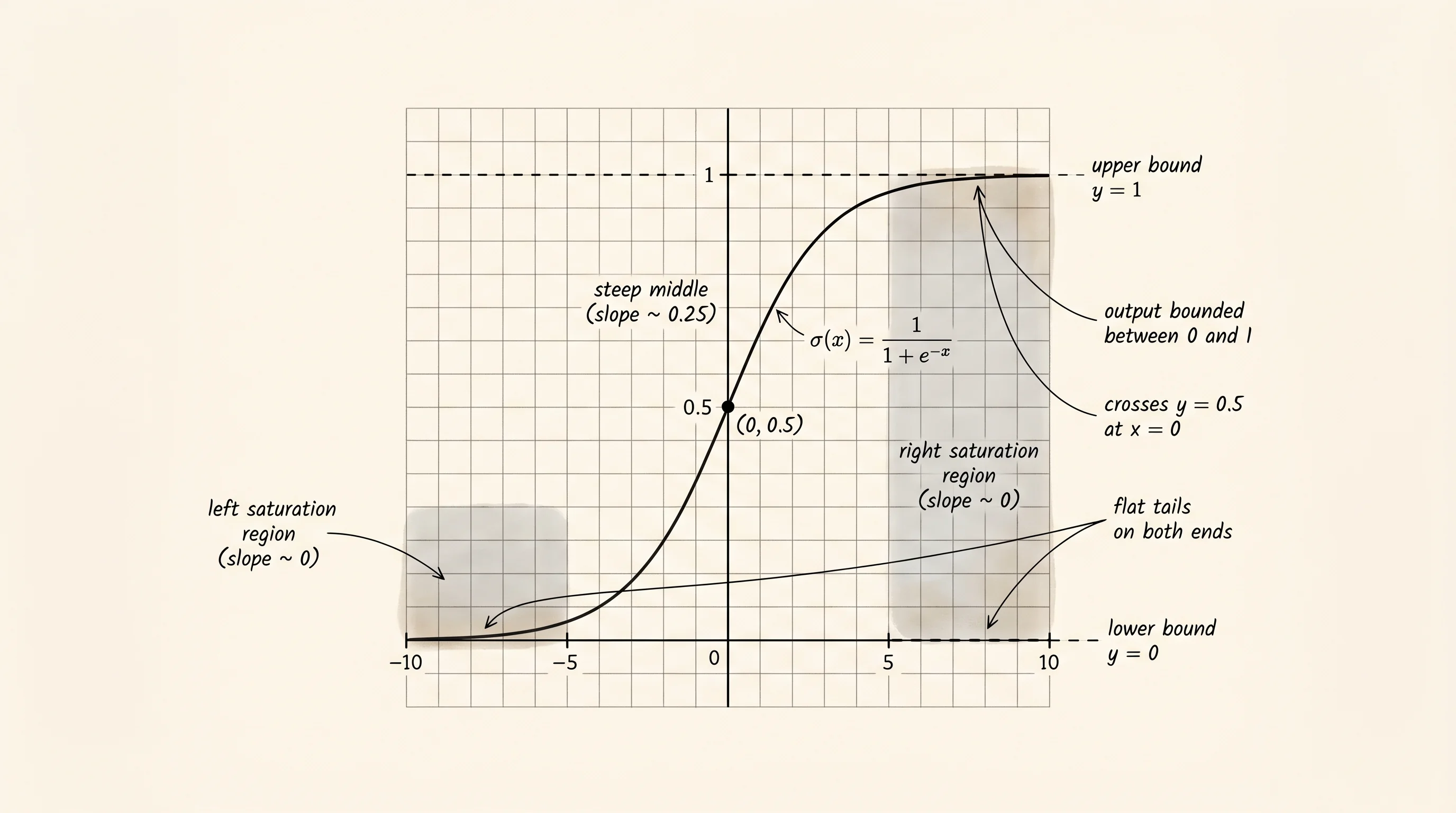
The function itself is small. Take a number x. Negate it. Raise e to that power. Add 1. Take the reciprocal. That is the sigmoid, written sigma(x) = 1 / (1 + e^(-x)). Plug in 0 and the e^0 in the denominator is 1, so sigma(0) = 1 / 2. Plug in a big positive number like 10 and e^(-10) is almost 0, so the denominator is almost 1 and sigma(10) is almost 1. Plug in -10 and e^(10) is around 22000, so the denominator is huge and sigma(-10) is almost 0. The curve glides smoothly from 0 on the left to 1 on the right, crossing 0.5 in the middle. Open sigmoid.py.

import math
 
 
def sigmoid(x):
    if x >= 0.0:
        return 1.0 / (1.0 + math.exp(-x))
    expo = math.exp(x)
    return expo / (1.0 + expo)

The two branches are the same function written two ways. Python's math.exp overflows for big positive arguments and the unsplit version 1 / (1 + math.exp(-x)) blows up when x is around -700. The trick is to feed math.exp only non-positive numbers. For non-negative x, exponentiate -x. For negative x, exponentiate x and rearrange. Same answer, no overflow.

A neural network needs more than the function. It needs the function's slope, because gradient descent steps in the direction the slope tells it to. The slope of the sigmoid has a tidy closed form, and the derivation is short enough to do here on the page. Let s be sigma(x) and let u be the denominator 1 + e^(-x), so s = 1 / u. The chain rule says ds/dx = (ds/du) _ (du/dx). The first piece is -1 / u^2. The second piece is the derivative of 1 + e^(-x), which is -e^(-x). Multiply them and the two negatives become a positive: ds/dx = e^(-x) / u^2. Now the algebra trick. Multiply the top by 1, written as e^x / e^x. The numerator becomes e^(-x) _ e^x / e^x = 1 / e^x, but it is cleaner to do it the other way: factor out one copy of u. Notice that e^(-x) = u - 1 (because u = 1 + e^(-x) by definition, so e^(-x) = u - 1). Substitute and ds/dx = (u - 1) / u^2 = 1/u - 1/u^2 = s - s^2 = s * (1 - s). The derivative of the sigmoid is the sigmoid times one minus the sigmoid. No new exponential to compute — once you have s, you have s'.

def sigmoid_derivative(x):
    s = sigmoid(x)
    return s * (1.0 - s)

Two lines. Trust nothing. Verify the analytical formula against finite differences — the wiggling trick from the neuron lesson. For each x, ask the analytical formula for the slope, then ask (sigmoid(x + eps) - sigmoid(x - eps)) / (2 * eps) for a numerical slope, and check that they agree.

def finite_difference(f, x, eps=1e-5):
    return (f(x + eps) - f(x - eps)) / (2.0 * eps)
 
 
for x in [-10.0, -5.0, -1.0, 0.0, 1.0, 5.0, 10.0]:
    analytic = sigmoid_derivative(x)
    numeric = finite_difference(sigmoid, x)
    print(f"x = {x:>5.1f}    analytic = {analytic:.6f}    numeric = {numeric:.6f}")

Run it and the two columns line up to six decimal places. The analytical formula is correct. From here on, every gradient through a sigmoid uses s * (1 - s) and never needs to recompute an exponential.

The S shape is the same shape Verhulst drew. Build a LogisticGrowthModel and watch it. Carrying capacity K is the ceiling. Growth rate r is how fast the colony moves toward the ceiling. Initial population P0 is the starting count. The closed-form solution to Verhulst's differential equation is P(t) = K / (1 + ((K - P0) / P0) _ e^(-r _ t)) — a sigmoid in disguise.

class LogisticGrowthModel:
    def __init__(self, carrying_capacity, growth_rate, initial):
        self.carrying_capacity = carrying_capacity
        self.growth_rate = growth_rate
        self.initial = initial
 
    def population_at(self, t):
        k = self.carrying_capacity
        p0 = self.initial
        ratio = (k - p0) / p0
        return k / (1.0 + ratio * math.exp(-self.growth_rate * t))

A petri dish with K = 1000 cells, r = 1.2 per hour, starting from a single cell, traces this when you sample the population every hour for 12 hours and plot it as ASCII.

  999.9 |                                                  *
  909.0 |                         *************************
  818.1 |                      ***
  727.2 |                     *
  636.3 |                   **
  545.4 |                  *
  454.5 |                 *
  363.6 |               **
  272.7 |              *
  181.8 |            **
   90.9 |         ***
    0.0 | ********
         +--------------------------------------------------
          t=0.0                                      t=12.0

Flat at the bottom, then the climb, then the ceiling. The same shape Pearl and Reed published for the United States population. The same shape a new social network draws as it spreads through a school. The same shape, rotated and shifted, that a sigmoid neuron draws across its input. The function is universal because the underlying logic — go fast when there is room, slow down as the room runs out — is universal.

Now wire the same function into a neuron. A SigmoidNeuron has one weight w, one bias b, and a forward pass that computes z = w _ x + b and returns sigma(z). Train it on a 1D classification task: 40 points clustered on the negative side of zero with label 0, and 40 points on the positive side with label 1. The neuron's job is to learn a w and b such that the curve sigma(w _ x + b) crosses 0.5 right between the two clusters.

class SigmoidNeuron:
    def __init__(self, weight=0.0, bias=0.0):
        self.weight = weight
        self.bias = bias
 
    def forward(self, x):
        return sigmoid(self.weight * x + self.bias)
 
    def gradient(self, x, y):
        z = self.weight * x + self.bias
        prediction = sigmoid(z)
        slope_z = sigmoid_derivative(z)
        error = prediction - y
        grad_w = 2.0 * error * slope_z * x
        grad_b = 2.0 * error * slope_z
        return grad_w, grad_b

The gradient lines come from the chain rule applied to squared error. Loss L = (p - y)^2 with p = sigma(z) and z = w _ x + b. Differentiating, dL/dw = 2 _ (p - y) _ sigma'(z) _ x and dL/db = 2 _ (p - y) _ sigma'(z). The sigma'(z) factor in the middle is the same s * (1 - s) we just derived.

def train_neuron(neuron, data, labels, learning_rate, epochs):
    for epoch in range(epochs):
        for x, y in zip(data, labels):
            grad_w, grad_b = neuron.gradient(x, y)
            neuron.weight -= learning_rate * grad_w
            neuron.bias -= learning_rate * grad_b

Run training for 200 epochs and the neuron locks onto the gap between the two clouds. The boundary is the x where w * x + b = 0, which solves to x = -b / w. Print the data with 0 and 1 markers, the boundary as |, and watch.

before training:
-------00000-00000000--------|--------111111111-1111--------
 -3.78                                                  3.77
boundary x = -0.000
 
after training:
-------00000-00000000--------|--------111111111-1111--------
 -3.78                                                  3.77
boundary x = -0.003

The boundary lands within a few thousandths of zero, exactly where the gap sits. The neuron learned a separator on a number line by following the slope of the sigmoid.

Now the problem. Print sigmoid and its derivative at the five interesting points.

for x in [-10.0, -5.0, 0.0, 5.0, 10.0]:
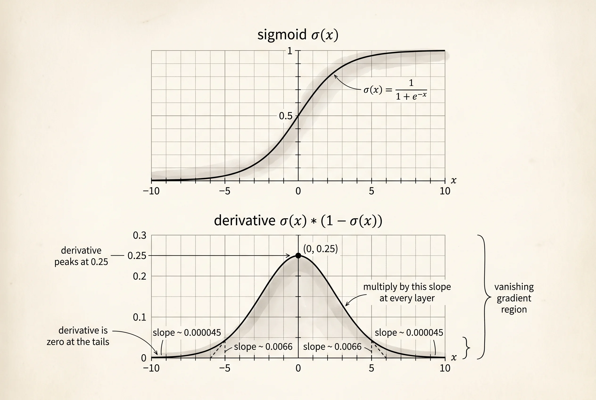
    print(f"x = {x:>5.1f}    sigmoid(x) = {sigmoid(x):.6f}    sigmoid'(x) = {sigmoid_derivative(x):.6f}")

x = -10.0    sigmoid(x) = 0.000045    sigmoid'(x) = 0.000045
x =  -5.0    sigmoid(x) = 0.006693    sigmoid'(x) = 0.006648
x =   0.0    sigmoid(x) = 0.500000    sigmoid'(x) = 0.250000
x =   5.0    sigmoid(x) = 0.993307    sigmoid'(x) = 0.006648
x =  10.0    sigmoid(x) = 0.999955    sigmoid'(x) = 0.000045

The derivative peaks at 0.25 in the middle and collapses toward zero at both ends. At x = 10 the slope is 0.000045 — four-and-a-half millionths. Backprop multiplies a gradient by this slope at every sigmoid layer it passes through. Stack ten sigmoid layers and feed in any input that pushes the pre-activation toward 10, and the gradient that reaches the first layer is multiplied by 0.000045 ten times in a row, which is a number with 43 zeros after the decimal point. The signal that should tell the early layers how to adjust their weights arrives as nothing. The early layers stop learning. This is the vanishing gradient problem, and the table above is the cause of it printed in plain numbers.

That table killed the sigmoid as a hidden activation. In 2012 Alex Krizhevsky's network for the ImageNet contest used ReLU instead of sigmoid in its hidden layers and won by such a margin that the entire field switched within a year. The sigmoid did not disappear — it still sits at the output of every binary classifier (where you actually want a probability between 0 and 1) and inside every LSTM gate (where you want a smooth on/off knob between 0 and 1). It just stopped being the default in the middle of a deep network. The shape that explained populations, viruses, and adoption curves still does that job perfectly. It only failed when stacked.

Sigmoid outputs are always positive, which makes every gradient step lean the same direction; centering the curve around zero makes training faster.