Tanh and Zero-Centering

Sigmoid pours every output into the bucket between 0 and 1. The bucket has no negative half. Whatever a neuron says about the world, it says with a positive number. That bias warps the gradient — every weight downstream of that neuron sees only positive signals coming in, so the gradient updates can only push the weights as a group in one direction at a time. The fix is to slide the whole curve down so it ranges from −1 through 0 to +1. The S-shape stays. The center moves to zero. The function is called the hyperbolic tangent, and its short name is tanh.

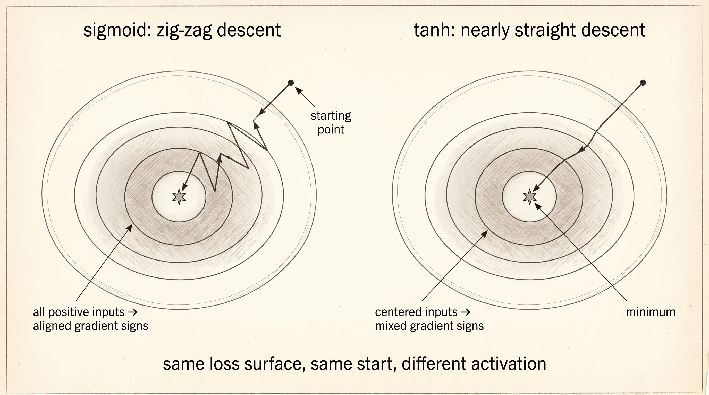
Yann LeCun wrote the case for tanh in a 1998 paper called Efficient BackProp. He had been training neural networks since the late 1980s — the convolutional net that read postal codes for the United States Postal Service was his — and he had measured the same thing over and over: tanh hidden layers trained faster than sigmoid hidden layers on the same problem. The reason was the centering. When the activations average to zero, the gradient steps point in cleaner directions. When they average to 0.5, the steps zigzag. A year before LeCun's paper, Sepp Hochreiter and Jürgen Schmidhuber had published the LSTM, the recurrent network architecture that would dominate sequence modeling for the next 18 years, and tanh became the standard activation inside the LSTM cell. Through the deep learning revival of the 2000s, tanh was the default. Then in 2012 a network called AlexNet swept an image contest using a different activation called ReLU, and tanh lost the hidden-layer crown. It still lives on inside LSTM cell-state updates, where the bounded range matters more than the speed.

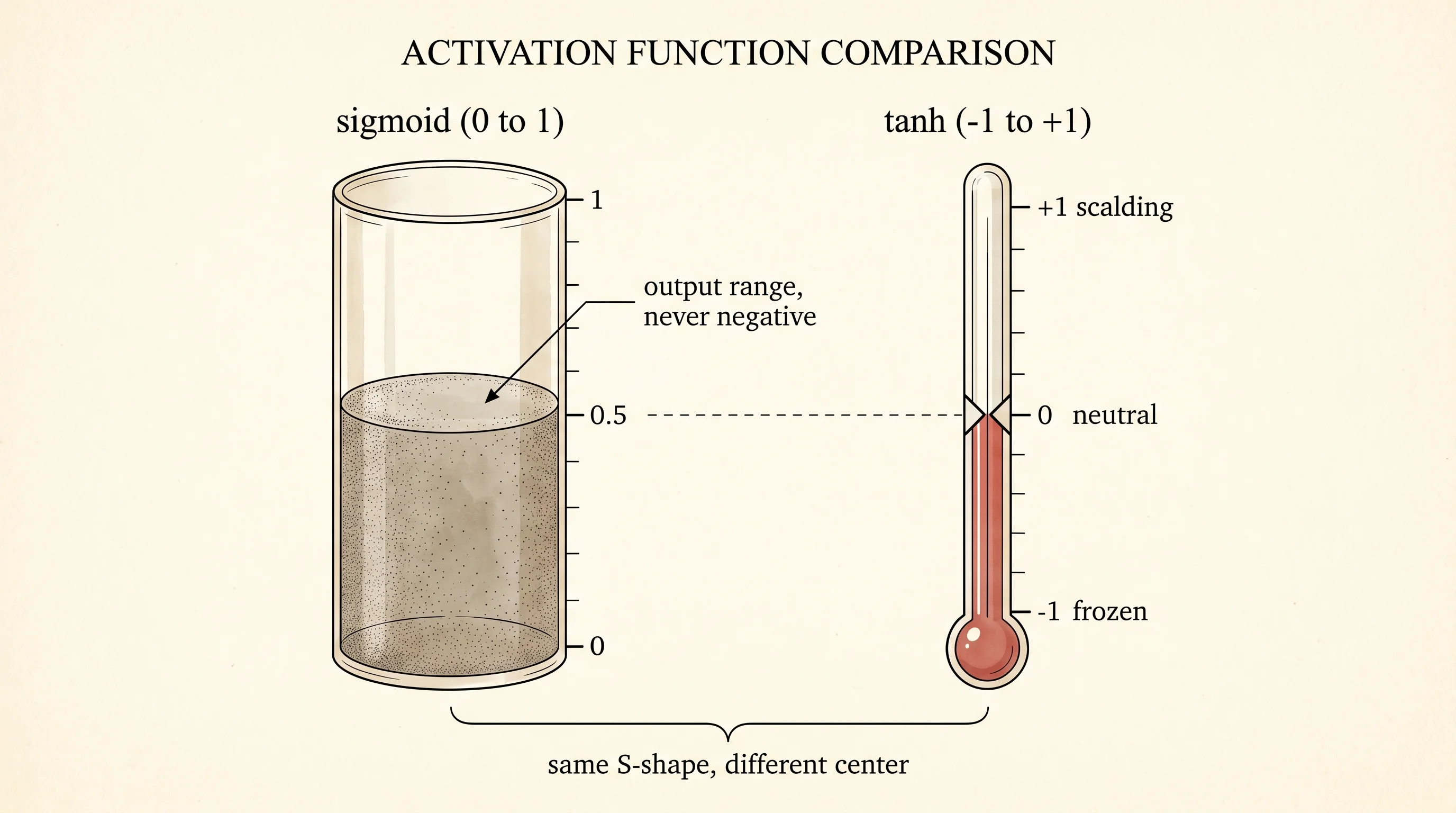
Switch the petri dish for a thermometer. Sigmoid was a population growing in a dish — it can grow but never shrink, so the reading is always positive. Tanh is a thermometer. It runs from frozen at −1 through a neutral 0 to scalding at +1. The middle reading is the upgrade. A neuron whose output can be negative is a neuron that can vote either way: yes, no, or stay quiet. Sigmoid only ever votes yes-with-some-confidence.

The math. Tanh is built from two exponentials, one for positive input and one for negative.

import math
 
 
def tanh(x):
    if x > 20.0:
        return 1.0
    if x < -20.0:
        return -1.0
    e_pos = math.exp(x)
    e_neg = math.exp(-x)
    return (e_pos - e_neg) / (e_pos + e_neg)
 
 
print(tanh(-2.0), tanh(0.0), tanh(2.0))

Run it.

-0.9640275800758169 0.0 0.9640275800758169

Three numbers tell the whole story. At x = 0 the curve passes through 0. At x = 2 the output is already 0.96 — most of the way to the ceiling. At x = −2 the output is the mirror image, −0.96. The two clamps near the top of the function catch values where exp would overflow. The function is symmetric around the origin: tanh(−x) = −tanh(x). Sigmoid had no such symmetry.

Tanh is a rescaled sigmoid. Specifically, tanh(x) = 2·σ(2x) − 1. Stretch sigmoid horizontally to make it twice as steep, then double its height to span 2 instead of 1, then subtract 1 to slide the bottom from 0 down to −1. Same S-shape, recentered. The fact that the two functions are this closely related is why the math of training a tanh network is the same as the math of training a sigmoid network — only the numbers shift.

The derivative is short and the proof is short. Write tanh(x) = (eˣ − e⁻ˣ) / (eˣ + e⁻ˣ). The quotient rule says the derivative equals the bottom times the derivative of the top, minus the top times the derivative of the bottom, all divided by the bottom squared. The derivative of the top is eˣ + e⁻ˣ, which is the bottom itself. The derivative of the bottom is eˣ − e⁻ˣ, which is the top itself. Multiply it out and the bottom-squared terms cancel into 1 minus (top/bottom)², which is 1 − tanh(x)².

def tanh_derivative(x):
    t = tanh(x)
    return 1.0 - t * t
 
 
for x in [-3.0, -1.0, 0.0, 1.0, 3.0]:
    print(f"x={x:+.1f}  tanh={tanh(x):+.4f}  d/dx={tanh_derivative(x):.4f}")

x=-3.0  tanh=-0.9951  d/dx=0.0099
x=-1.0  tanh=-0.7616  d/dx=0.4200
x=+0.0  tanh=+0.0000  d/dx=1.0000
x=+1.0  tanh=+0.7616  d/dx=0.4200
x=+3.0  tanh=+0.9951  d/dx=0.0099

The derivative hits 1.0 at the center and falls toward 0 at the tails. Compare that peak to sigmoid's peak derivative of 0.25. Tanh passes four times more gradient through at the middle. That extra gradient is half of why training is faster. The other half is the centering, which is what the rest of the lesson measures.

Generate a signal to push through the network. A waveform — a sum of sine waves — gives a varied input that has both positive and negative samples, the kind of thing a microphone or a sensor would produce.

def generate_waveform(n_points, frequencies):
    samples = []
    for index in range(n_points):
        t = index / n_points
        value = 0.0
        for frequency in frequencies:
            value += math.sin(2.0 * math.pi * frequency * t)
        samples.append(value / len(frequencies))
    return samples
 
 
waveform = generate_waveform(n_points=400, frequencies=[2.0, 5.0, 11.0])
print(waveform[:5])

[0.0, 0.2855..., 0.4923..., 0.5187..., 0.3601...]

Four hundred samples that wiggle between roughly −1 and +1. Slide a window 16 samples wide across the waveform and feed each window through a 5-layer network. Build two networks with the same shape — the same layer sizes, the same random seed for the weights — so the only difference is the activation function.

To watch what happens inside, attach an ActivationTracker that records every neuron's output at every layer for every window. The tracker keeps the raw numbers and reports the mean, the standard deviation, the min, and the max for each layer.

class ActivationTracker:
    def __init__(self, n_layers):
        self.samples_per_layer = [[] for _ in range(n_layers)]
 
    def record(self, layer_index, activations):
        self.samples_per_layer[layer_index].extend(activations)
 
    def layer_stats(self, layer_index):
        values = self.samples_per_layer[layer_index]
        average = sum(values) / len(values)
        variance = sum((v - average) ** 2 for v in values) / len(values)
        return {
            "mean": average,
            "std": math.sqrt(variance),
            "min": min(values),
            "max": max(values),
        }

The tracker is dumb on purpose. Every forward pass calls record once per layer with the layer's outputs, and at the end the tracker can hand back the four statistics that summarize the layer's behavior across the whole signal.

Wire two networks side by side. Same seed, same architecture, two activations.

random.seed(7)
sigmoid_network = build_network(sigmoid, [16, 12, 12, 12, 12, 1])
random.seed(7)
tanh_network = build_network(tanh, [16, 12, 12, 12, 12, 1])
 
sigmoid_tracker = ActivationTracker(5)
tanh_tracker = ActivationTracker(5)
 
for start in range(len(waveform) - 16 + 1):
    window = waveform[start : start + 16]
    forward_with_tracking(sigmoid_network, window, sigmoid_tracker)
    forward_with_tracking(tanh_network, window, tanh_tracker)

The window slides 385 times. Each slide produces 12 outputs at layers 1–4 and 1 output at layer 5. Multiply that out and the tracker holds tens of thousands of numbers per layer, more than enough to estimate the mean and the standard deviation reliably. Print the comparison table.

layer |  sigmoid_mean |  sigmoid_std |  tanh_mean |  tanh_std
-------------------------------------------------------------
    1 |        0.5003 |       0.0880 |    +0.0014 |    0.3183
    2 |        0.5148 |       0.1286 |    +0.0019 |    0.3134
    3 |        0.5013 |       0.1509 |    +0.0009 |    0.2999
    4 |        0.5175 |       0.1462 |    -0.0001 |    0.2686
    5 |        0.4646 |       0.0003 |    +0.0015 |    0.1729

Read it column by column. The sigmoid means sit a hair above 0.5 in every layer. The tanh means sit a hair on either side of 0. That is the centering. It is not a metaphor and it is not a chart — it is five numbers each, printed in a column, and the difference is impossible to miss. The sigmoid network's downstream layers are receiving inputs that all live in a half-space. The tanh network's downstream layers are receiving inputs that span both halves of the number line.

Why does this matter for training? When all the inputs to a neuron are positive, the gradient with respect to every one of that neuron's weights gets multiplied by the same sign. Every weight in the row gets pushed up together or down together. The optimizer cannot move some weights up while moving others down in the same step, so the path from start to a good answer becomes a zigzag. With centered activations the inputs come in with mixed signs, the gradient signs mix too, and the weights can move independently. The same number of steps covers more ground.

Look at the std column in layer 5. Sigmoid's std collapses to 0.0003 — every output is essentially the same number. Tanh's std at layer 5 is 0.1729, six hundred times larger. Sigmoid is collapsing the signal as it flows deeper. Tanh is preserving variation. A network whose final layer outputs the same number for every input has nothing to learn from. A network whose final layer still varies has signal to grade and a gradient to follow.

Question for the reader: in a single layer, which activation will produce a wider spread of outputs given the same incoming signal — the one that maps every real number into a bucket of width 1 (sigmoid), or the one that maps every real number into a bucket of width 2 (tanh)? Look at the std columns. Tanh wins in the early layers because its output range is twice as tall. Same neurons, same weights, twice the room to vary.

Tanh has one weakness it shares with sigmoid. At the tails of the curve, the derivative goes to zero. Look back at the derivative table — at x = ±3 the slope is already 0.0099, and at x = ±5 it is essentially zero. A neuron whose pre-activation drifts deep into the saturated region passes almost no gradient, so its weights stop updating. A 5-layer network with all layers saturated has a vanishing gradient at the input — the same problem sigmoid has, just shifted. The next lesson introduces an activation function that refuses to saturate at all on the positive side.