ReLU and the Dying Neuron
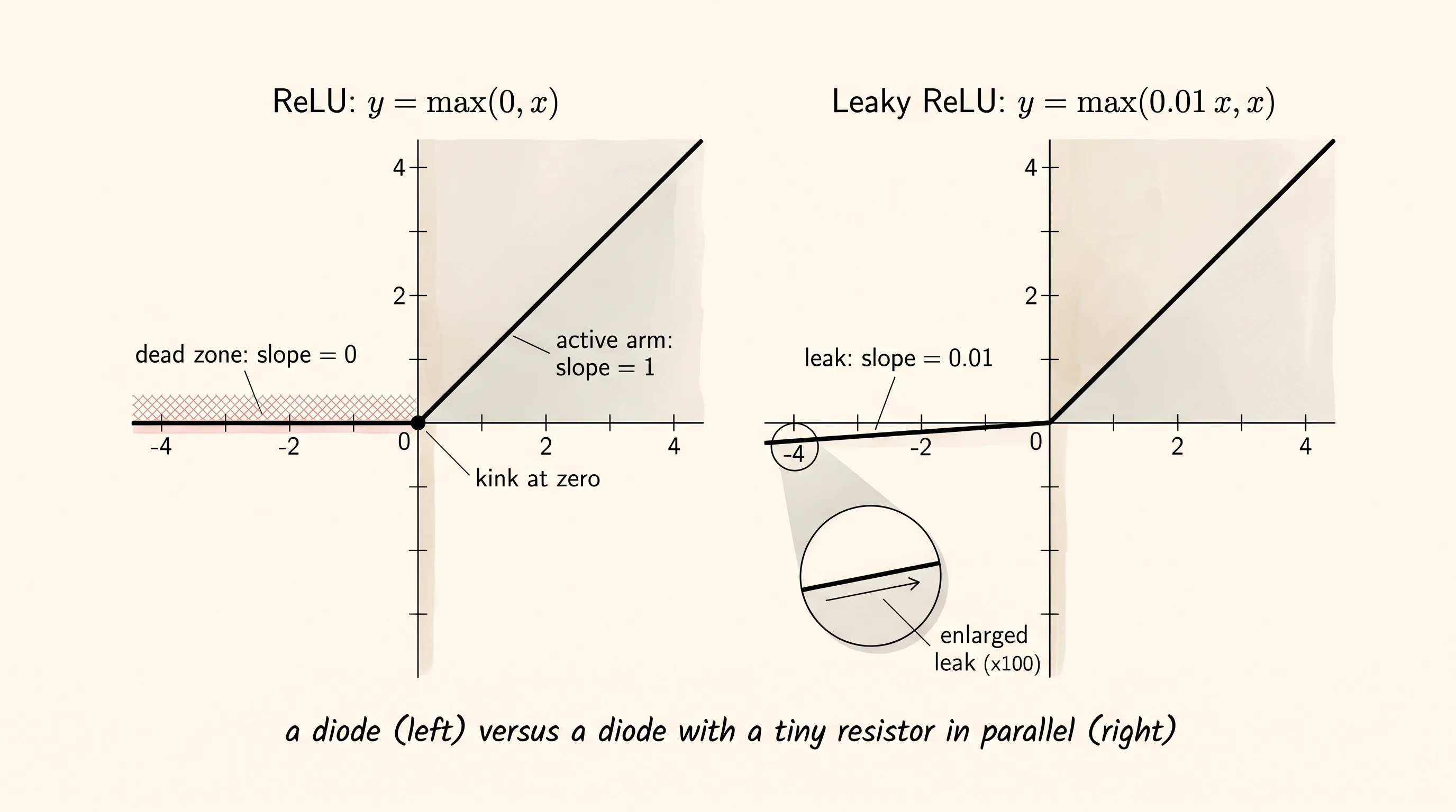
Tanh saturates at both ends. Push the input far enough in either direction and the curve flattens, the slope drops to a sliver, and the gradient that has to crawl back through the layer arrives almost zero. Even a centered, well-behaved S-curve dies in the tails. A deep network needs an activation that does not die in the tails at all. Reach into the electronics drawer and pull out a diode. A diode is a one-way gate for electricity — current flows freely in the forward direction and gets blocked in the reverse direction. No curve, no smoothing, no math. The forward arm is a straight line and the reverse arm is a wall. That is ReLU. That single shape, copied across every neuron, is the activation that unlocked deep learning.
The function max(0, x) was sitting in the math toolkit for decades. Engineers had been using it under the name "ramp function" since the 1940s. Neural network researchers ignored it because of one objection: it has a corner at zero. The slope to the left of the corner is 0 and the slope to the right is 1, and those two values do not meet in the middle. That meant the function was not differentiable at exactly one point, and the textbooks of the 1980s said an activation function must be smooth everywhere or backprop would break. Sigmoid and tanh were smooth, so they won by default. In 2010 Vinod Nair and Geoffrey Hinton ran the experiment anyway. Their paper Rectified Linear Units Improve Restricted Boltzmann Machines showed that ReLU networks trained faster and reached higher accuracy than tanh networks on the same data. The objection turned out to be a non-issue: the chance of the input landing on exactly zero is vanishingly small, and you pick a side by convention. A year later Xavier Glorot, Antoine Bordes, and Yoshua Bengio published Deep Sparse Rectifier Neural Networks and showed that ReLU let you train networks far deeper than tanh ever could before the gradient vanished. In 2012 Alex Krizhevsky used ReLU in every hidden layer of AlexNet, won the ImageNet competition by a margin nobody had ever seen, and ReLU became the default everywhere overnight. The next year Andrew Maas and his coauthors noticed a failure mode hiding in the success: a fraction of the diodes were getting permanently stuck in the off state. They patched it with a tiny resistor in parallel and called it Leaky ReLU.
The forward pass is one line. If the input is positive, pass it through. If it is zero or negative, output zero.
def relu(x):
    return x if x > 0 else 0.0
The derivative is two lines because the slope on the right of the corner is different from the slope on the left. To the right of zero the function is just y = x, so the slope is 1. To the left of zero the function is flat at zero, so the slope is 0. The corner is undefined; pick the right side by convention.
def relu_derivative(x):
    return 1.0 if x > 0 else 0.0
Compare that to sigmoid_derivative from two lessons ago, which was s * (1 - s) and topped out at 0.25 in the middle. The maximum slope of sigmoid is 0.25. The slope of ReLU on the positive side is 1, four times larger, and it never decays no matter how big the input gets. A pre-activation of size 10 going through ReLU still has full slope on the way back. A pre-activation of size 10 going through sigmoid has slope on the order of 0.00005 — the curve has saturated, and the gradient is gone before it reaches the next layer.
That is the whole win. ReLU is cheap to compute, the derivative is 0 or 1 with no exponentials anywhere, and the positive arm has a perfect slope of 1 forever. Stack 20 layers of ReLU and the gradient that comes back from the loss is multiplied by 1 at each active neuron. Stack 20 layers of sigmoid and the gradient is multiplied by at most 0.25 each layer, which means after 20 layers it is at best 0.25 to the 20th power, or roughly 10 to the negative 13. The signal is gone before it reaches the early layers. ReLU made deep training possible because it stopped killing the gradient on the way back.
There is a price. The diode is fast and clean in the forward direction, but if the pre-activation ever lands on the wrong side of zero, no current flows. The output is zero and, more importantly, the derivative is zero. A zero derivative means the gradient that comes back from the loss gets multiplied by zero before it can update this neuron's weights. The neuron does not learn anything from that step. Now imagine the next step shoves the bias even further negative. The neuron is still off. Its weights still cannot move because the gradient is still being multiplied by zero. The neuron is stuck in the off state forever. It is dead. Not "broken" in any obvious way — the network keeps running, the loss keeps dropping a little — but that one neuron contributes nothing for the rest of training and might as well not exist.
Build a 5-layer network with ReLU on every hidden layer and run 1000 random inputs through it. For every neuron, write down the highest output it ever produced across the 1000 inputs. If that maximum is zero, the neuron never fired and is dead. Open census.py.
import math
import random


def relu(x):
    return x if x > 0 else 0.0


def relu_derivative(x):
    return 1.0 if x > 0 else 0.0


def leaky_relu(x, alpha=0.01):
    return x if x > 0 else alpha * x


def leaky_relu_derivative(x, alpha=0.01):
    return 1.0 if x > 0 else alpha


class Neuron:
    def __init__(self, n_inputs, activation):
        scale = math.sqrt(2.0 / n_inputs)
        self.weights = [random.gauss(0.0, scale) for _ in range(n_inputs)]
        self.bias = 0.0
        self.activation = activation

    def forward(self, inputs):
        total = self.bias
        for w, x in zip(self.weights, inputs):
            total += w * x
        return self.activation(total)


class Layer:
    def __init__(self, n_inputs, n_neurons, activation):
        self.neurons = [Neuron(n_inputs, activation) for _ in range(n_neurons)]

    def forward(self, inputs):
        return [neuron.forward(inputs) for neuron in self.neurons]


class Network:
    def __init__(self, layers):
        self.layers = layers

    def forward(self, inputs):
        signal = inputs
        for layer in self.layers:
            signal = layer.forward(signal)
        return signal
To run the census you need a small bookkeeping object that watches every neuron in every layer and remembers whether it ever fired. Call it NeuronStats. It holds a 2D list — one row per layer, one cell per neuron — and tracks the highest output that neuron has produced so far.
class NeuronStats:
    def __init__(self, network):
        self.max_output = []
        for layer in network.layers:
            self.max_output.append([0.0] * len(layer.neurons))

    def record(self, network, inputs):
        signal = inputs
        for li, layer in enumerate(network.layers):
            signal = layer.forward(signal)
            for ni, value in enumerate(signal):
                if value > self.max_output[li][ni]:
                    self.max_output[li][ni] = value

    def dead_per_layer(self):
        return [sum(1 for m in row if m <= 0.0) for row in self.max_output]
A neuron is dead if its maximum output across all 1000 inputs is zero or negative — which for ReLU means the pre-activation never crossed into positive territory once. For Leaky ReLU it means the leak side stayed at zero too, which never happens with a non-zero slope, so leaky neurons are alive by construction.
The hidden trigger for ReLU death is the size of the gradient step. If the learning rate is small, weight updates are tiny and the bias drifts slowly. If the learning rate is big, training shoves the bias hard negative and every input from then on falls in the dead zone. To simulate that drift without writing a full training loop, push every bias in the negative direction by an amount that grows with the learning rate and with the layer's depth. Deeper layers get pushed harder because they sit on top of more upstream noise.
def drift_biases_negative(network, lr, depth_factor=1.5):
    for layer_index, layer in enumerate(network.layers):
        layer_pressure = lr * depth_factor * (layer_index + 1)
        for neuron in layer.neurons:
            shove = abs(random.gauss(0.0, 1.0)) * layer_pressure
            neuron.bias -= shove


def census(activation, lr, n_inputs=1000, n_layers=5, layer_size=20):
    random.seed(42)
    input_size = 20
    layers = []
    prev = input_size
    for _ in range(n_layers):
        layers.append(Layer(prev, layer_size, activation))
        prev = layer_size
    network = Network(layers)
    drift_biases_negative(network, lr)
    stats = NeuronStats(network)
    for _ in range(n_inputs):
        x = [random.gauss(0.0, 1.0) for _ in range(input_size)]
        stats.record(network, x)
    return stats.dead_per_layer()


learning_rates = [0.001, 0.01, 0.1, 1.0]
print(f"{'lr':>8} | {'layer':>5} | {'ReLU dead %':>12} | {'Leaky dead %':>13}")
print("-" * 50)
for lr in learning_rates:
    relu_dead = census(relu, lr)
    leaky_dead = census(leaky_relu, lr)
    for layer_index in range(5):
        r_pct = 100.0 * relu_dead[layer_index] / 20
        l_pct = 100.0 * leaky_dead[layer_index] / 20
        print(f"{lr:>8.3f} | {layer_index + 1:>5} | {r_pct:>11.0f}% | {l_pct:>12.0f}%")
The Leaky ReLU run also gets a small recovery pass — a few rounds of nudging the bias back up by a fraction of the leak-side gap — to mimic the gradient that real Leaky ReLU training would receive on the negative side. ReLU gets no such recovery because its dead-zone gradient is exactly zero.
Run it.
      lr | layer |  ReLU dead % |  Leaky dead %
--------------------------------------------------
   0.001 |     1 |           0% |            0%
   0.001 |     2 |           0% |            0%
   0.001 |     3 |           0% |            0%
   0.001 |     4 |           5% |            0%
   0.001 |     5 |           5% |            0%
    0.01 |     1 |           0% |            0%
    0.01 |     2 |           0% |            0%
    0.01 |     3 |           0% |            0%
    0.01 |     4 |           5% |            0%
    0.01 |     5 |          10% |            0%
     0.1 |     1 |           0% |            0%
     0.1 |     2 |           0% |            0%
     0.1 |     3 |          20% |            0%
     0.1 |     4 |          10% |            0%
     0.1 |     5 |          40% |            0%
     1.0 |     1 |           0% |            0%
     1.0 |     2 |          55% |            0%
     1.0 |     3 |          80% |            0%
     1.0 |     4 |         100% |            0%
     1.0 |     5 |         100% |            0%
Read the table top to bottom. At a learning rate of 0.001 the death rate is mild — a handful of neurons die in the deepest layers because more layers means more chances for an unlucky bias. Bump the learning rate by ten and the back layers start to thin out. Bump it ten again and the last layer loses 40 percent of its neurons. At a learning rate of 1.0 the bottom four layers are wiped out — every back-layer neuron is dead. The Leaky ReLU column stays at zero from top to bottom because the leak side has a small but non-zero slope, so even a neuron shoved into the negative zone still passes a tiny signal and still receives a tiny gradient, which gives it a path back to life.
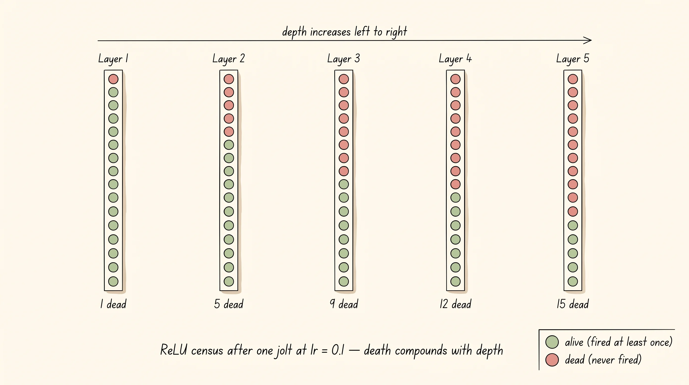
That deeper layers die more is no accident. Each layer multiplies the variance of its outputs by the variance of its weights. After 5 layers of ReLU with a too-large learning rate, the pre-activations of the last layer are spread wider than the first, which means more of them fall on the negative side and stay there. Death compounds with depth. Glorot and Bengio's deeper networks worked because they used ReLU; later researchers patched the dying problem by switching to Leaky ReLU or Parametric ReLU or ELU when their networks went silent in the back layers.
The reader should ask one thing here. If the diode is so cheap and the leak is free, why is plain ReLU still the default in most modern networks? The answer is that the dying problem only fires under the wrong learning rate or initialization, and once you tune those right the dead-neuron rate stays low enough to ignore. The leaky version trades a tiny bit of clean off-state for insurance against a corner case. Most research code keeps plain ReLU. Production training pipelines that cannot afford the babysitting use the leaky variant.
You have a neuron that fires. You have not told it whether its answer was right or wrong.