The Loss Surface
A neuron fires. It says a number. The number is wrong, or it is right, or it is right by accident — and the neuron has no idea which. To teach it, you need a way to score every guess with a single number that gets small when the guess is good and big when the guess is bad. That number is the loss. Imagine a hiker dropped on a mountain in the dark with one instrument: an altimeter. The altimeter reads the elevation right under his feet. The lowest valley on the mountain is the answer. He cannot see the valley. He can only feel which way the ground tilts and step downhill. The shape of the mountain — smooth bowl, narrow ravine, plateau with a cliff — decides whether he reaches the valley in an hour or wanders for a week.
Adrien-Marie Legendre published the first version of this idea in 1805. He was an astronomer trying to fit an orbit to a few telescope readings of a comet. The readings disagreed with each other because every telescope is a little off. Legendre wrote down a rule: pick the orbit that makes the sum of the squared disagreements as small as possible. He called the method least squares and it solved his comet problem in an afternoon. Carl Friedrich Gauss in Germany said he had been using the same trick since 1795 to predict the position of the dwarf planet Ceres, and the two of them spent the next decade fighting in journals over who invented it. There was a third person in the room nobody listened to. Pierre-Simon Laplace had been quietly using a different rule for forty years — pick the orbit that makes the sum of the absolute disagreements as small as possible. His rule was just as reasonable and arguably more honest. It lost the math war anyway, because squared errors give you a clean equation you can solve with pen and paper, and absolute errors give you a kink at zero that breaks the algebra. Computers in 1805 were humans, and humans hate kinks. Two centuries later the same two losses are still in every deep learning library, and the only big addition is one custom loss per problem class — squared error for regression, cross-entropy for classification, and a zoo of bespoke losses for reinforcement learning where the answer is a strategy and not a number.

A loss is a function of the model's parameters. Not the data. The data is fixed — those are the comet readings, the photos in the training set, the rent prices in the spreadsheet. The parameters are the dials you turn. For a neuron with three inputs, the dials are the three weights and the bias. For a model the size of GPT-4, the dials number in the trillions. Every setting of the dials gets one loss number, computed by running every data point through the model with those dial settings and adding up how wrong each prediction was. Plot the loss over every possible dial setting and you get a landscape. The landscape lives in as many dimensions as you have dials. The hiker is not walking on a real mountain. He is walking on a mountain in 89-dimensional space (in the circle network from the last lesson) or 1.7-trillion-dimensional space (in GPT-4). The shape is what matters, and the shape comes from the choice of loss.
Pick a model small enough to draw. Two parameters. y = w1 · x + w2. A line, slope w1 and intercept w2. Generate 40 noisy points along the true line w1 = 1.5, w2 = 0.5. Now sweep w1 from -2 to 4 and w2 from -2 to 4 on a 21 by 21 grid. At every cell of the grid, compute the loss. The grid is the loss surface for this model on this data. Different losses give different surfaces.
The four losses you should know by name are mean squared error, mean absolute error, Huber, and hinge. Each one is a one-line formula on top of "prediction minus target." Write them as plain Python functions that take a list of predictions and a list of targets and return a single number.
def mse_loss(predictions, targets):
total = 0.0
for prediction, target in zip(predictions, targets):
error = prediction - target
total += error * error
return total / len(predictions)
def mae_loss(predictions, targets):
total = 0.0
for prediction, target in zip(predictions, targets):
total += abs(prediction - target)
return total / len(predictions)
def huber_loss(predictions, targets, delta=1.0):
total = 0.0
for prediction, target in zip(predictions, targets):
error = prediction - target
magnitude = abs(error)
if magnitude <= delta:
total += 0.5 * error * error
else:
total += delta * (magnitude - 0.5 * delta)
return total / len(predictions)
def hinge_loss(predictions, targets):
total = 0.0
for prediction, target in zip(predictions, targets):
margin = 1.0 - target * prediction
total += margin if margin > 0.0 else 0.0
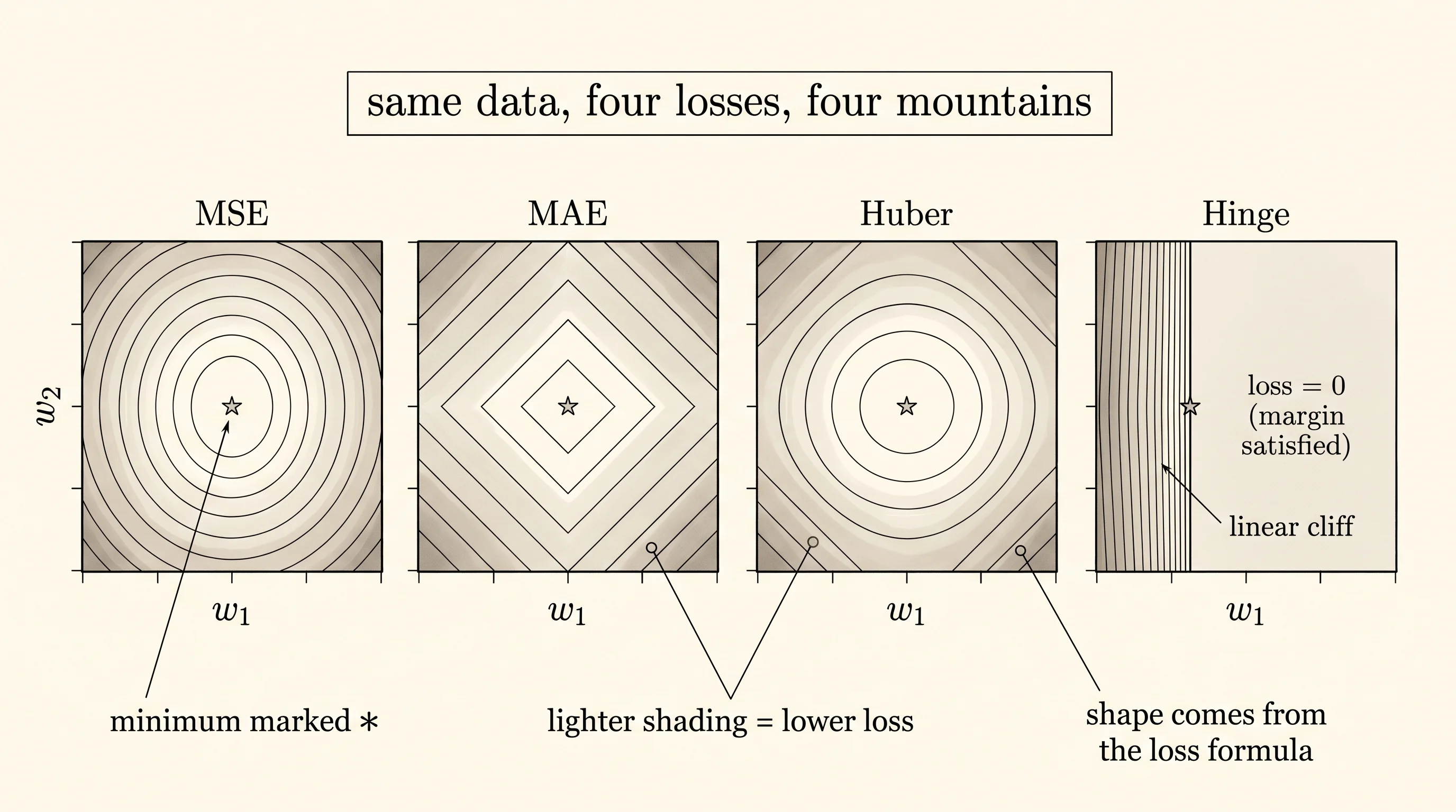
return total / len(predictions)MSE squares the error. A point that is off by 2 contributes 4 to the loss; a point off by 4 contributes 16. One bad outlier dominates everything. MAE takes the absolute value. Off by 2 contributes 2, off by 4 contributes 4. Every point gets a fair vote. Huber uses MSE near zero and switches to MAE once the error grows past delta — a smooth bowl in the middle, two straight ramps on the sides. Hinge is the odd one out. It is for classification, not regression. The target is +1 or -1 (not a number to fit, a side to be on). The loss is zero when the prediction lands on the right side by at least 1 — a free pass for confident correct answers. Otherwise it is linear. There is a wide flat region where the loss does not change at all, which makes the gradient zero and gradient descent freeze.
To draw the surface you need a sweep function that walks the grid and asks the loss for the loss at every cell.
def predict(w1, w2, xs):
    return [w1 * x + w2 for x in xs]


def compute_loss_surface(loss_fn, data, w1_range, w2_range, grid_size):
    xs = [x for x, _ in data]
    ys = [y for _, y in data]
    w1_low, w1_high = w1_range
    w2_low, w2_high = w2_range
    surface = []
    for row in range(grid_size):
        w2 = w2_low + (w2_high - w2_low) * row / (grid_size - 1)
        row_values = []
        for col in range(grid_size):
            w1 = w1_low + (w1_high - w1_low) * col / (grid_size - 1)
            predictions = predict(w1, w2, xs)
            row_values.append(loss_fn(predictions, ys))
        surface.append(row_values)
    return surface
The grid is a list of rows. Each row is a list of loss numbers. Now turn the grid into a picture. A contour map paints each cell with one of a few shading characters: light shading for low loss, heavy shading for high loss. Four bands is enough to read the shape. The Unicode block characters ░ ▒ ▓ █ are perfect — they go from sparse hatching to solid black in evenly spaced steps. Add a * over the cell with the smallest loss so the eye finds the valley.
def find_minimum(surface):
    best_row, best_col = 0, 0
    best_value = surface[0][0]
    for row, values in enumerate(surface):
        for col, value in enumerate(values):
            if value < best_value:
                best_value = value
                best_row, best_col = row, col
    return best_row, best_col, best_value


def ascii_contour(surface, levels=4):
    shades = [" ", "░", "▒", "▓", "█"]
    flat = [v for row in surface for v in row]
    low, high = min(flat), max(flat)
    span = high - low if high > low else 1.0
    min_row, min_col, _ = find_minimum(surface)
    rows = []
    for r, values in enumerate(surface):
        cells = []
        for c, value in enumerate(values):
            if r == min_row and c == min_col:
                cells.append("*")
                continue
            band = int((value - low) / span * levels)
            if band > levels:
                band = levels
            cells.append(shades[band])
        rows.append("".join(cells))
    return "\n".join(rows)
Wire it together. Generate two datasets — one for the regression losses (a noisy line) and one for the hinge loss (points labeled +1 or -1 by which side of a line they sit on). Compute four surfaces. Print them side by side.
import random

random.seed(11)

def generate_regression_data(n, true_w1, true_w2, noise_std):
    samples = []
    for _ in range(n):
        x = random.uniform(-1.0, 1.0)
        y = true_w1 * x + true_w2 + random.gauss(0.0, noise_std)
        samples.append((x, y))
    return samples


def generate_classification_data(n, true_w1, true_w2):
    samples = []
    for _ in range(n):
        x = random.uniform(-1.0, 1.0)
        label = 1.0 if true_w1 * x + true_w2 > 0.0 else -1.0
        samples.append((x, label))
    return samples


regression = generate_regression_data(40, 1.5, 0.5, 0.2)
classification = generate_classification_data(40, 1.5, 0.5)
huber = lambda p, t: huber_loss(p, t, delta=1.0)

losses = [
    ("MSE",   mse_loss,   regression),
    ("MAE",   mae_loss,   regression),
    ("Huber", huber,      regression),
    ("Hinge", hinge_loss, classification),
]

for name, loss_fn, data in losses:
    surface = compute_loss_surface(loss_fn, data, (-2.0, 4.0), (-2.0, 4.0), 21)
    print(name)
    print(ascii_contour(surface))
    print()
Run it. The four contour maps come out side by side and tell four different stories.
MSE                     MAE                     Huber                   Hinge
░░░░░░░░░░░░░░░░░░░░░   ▒░░░░▒▒▒▒▒▒▒▒▒▒▒▒▒▒▒▒   ░░░░░░░░░▒▒▒▒▒▒▒▒▒▒▒▒   ▓▓▓▓▓▓▒▒▒▒▒▒▒░░░░░░░░
░░░░          ░░░░░░░   ░░░░░░░░░░░▒▒▒▒▒▒▒▒▒▒   ░░░░░░░░░░░░░░░▒▒▒▒▒▒   ▓▓▓▓▒▒▒▒▒▒▒░░░░░░░░░
░░               ░░░░   ░░░░░░░░░░░░░░░░░░▒▒▒   ░░░░░░░░░░░░░░░░░░░░▒   ▓▓▓▒▒▒▒▒▒░░░░░░░
                   ░░   ░░░░░░░░░░░░░░░░░░░░░   ░░░░░░  ░░░░░░░░░░░░░   ▓▓▓▒▒▒▒░░░░░░░
                        ░░░░░░    ░░░░░░░░░░░   ░░░░           ░░░░░░   ▓▓▒▒▒▒░░░░░░
                        ░░░░░           ░░░░░   ░░░               ░░░   ▓▓▒▒▒▒░░░░
                        ░░░░              ░░░   ░░░                ░░   ▓▓▒▒▒▒░░░
                        ░░░░               ░░   ░░░                 ░   ▓▒▒▒▒░░░░
            *           ░░░░        *       ░   ░░░         *           ▓▒▒▒▒░░░░
                        ░░░░░               ░   ░░░░                    ▓▒▒▒░░░░
░                       ░░░░░░              ░   ░░░░░                   ▒▒▒▒░░░░░           *
░                       ░░░░░░░░            ░   ░░░░░░                  ▒▒▒▒░░░░░░
░░░                     ▒░░░░░░░░░░         ░   ░░░░░░░░                ▒▒▒▒░░░░░░░░
░░░░                    ▒▒▒░░░░░░░░░░░░░░░░░░   ▒▒░░░░░░░░░░        ░   ▒▒▒▒▒░░░░░░░░
░░░░░░                  ▒▒▒▒▒░░░░░░░░░░░░░░░░   ▒▒▒▒░░░░░░░░░░░░░░░░░   ▒▒▒▒▒▒▒░░░░░░░░
▒░░░░░░░░               ▒▒▒▒▒▒▒▒▒▒░░░░░░░░░░░   ▒▒▒▒▒▒░░░░░░░░░░░░░░░   ▓▒▒▒▒▒▒▒▒░░░░░░░░
▒▒▒░░░░░░░░░░     ░░░   ▒▒▒▒▒▒▒▒▒▒▒▒▒▒▒▒░░░░░   ▒▒▒▒▒▒▒▒▒▒▒▒░░░░░░░░░   ▓▓▒▒▒▒▒▒▒▒░░░░░░░░
▒▒▒▒▒░░░░░░░░░░░░░░░░   ▓▓▓▒▒▒▒▒▒▒▒▒▒▒▒▒▒▒▒▒▒   ▓▓▒▒▒▒▒▒▒▒▒▒▒▒▒▒▒▒▒░░   ▓▓▓▓▒▒▒▒▒▒▒▒░░░░░░░░
▓▒▒▒▒▒▒▒░░░░░░░░░░░░░   ▓▓▓▓▓▓▓▓▒▒▒▒▒▒▒▒▒▒▒▒▒   ▓▓▓▓▓▓▒▒▒▒▒▒▒▒▒▒▒▒▒▒▒   ▓▓▓▓▓▒▒▒▒▒▒▒▒▒░░░░░░░
▓▓▓▒▒▒▒▒▒▒▒▒░░░░░░░░░   ▓▓▓▓▓▓▓▓▓▓▓▓▓▓▒▒▒▒▒▒▒   ▓▓▓▓▓▓▓▓▓▓▓▓▒▒▒▒▒▒▒▒▒   ▓▓▓▓▓▓▓▒▒▒▒▒▒▒▒░░░░░░
█▓▓▓▓▓▒▒▒▒▒▒▒▒▒▒▒▒▒▒▒   █▓▓▓▓▓▓▓▓▓▓▓▓▓▓▓▓▓▓▓▓   █▓▓▓▓▓▓▓▓▓▓▓▓▓▓▓▓▓▓▒▒   █▓▓▓▓▓▓▓▓▒▒▒▒▒▒▒▒░░░░
MSE is a clean elliptical bowl. The lightest cells form a wide ring around the minimum. The hiker rolls a marble onto this surface anywhere and it ends up at the star. Every step downhill shrinks the loss; the slope points straight at the answer.
MAE has the same minimum but the basin around it is sharper. The light region is a cross-shaped ravine that follows the two axes. Walk perpendicular to the ravine and the loss drops fast; walk along the ravine and you barely move. The kink at every individual error becomes a kink at the whole-surface scale. Computers handle the kink fine, which is why MAE is back in fashion, but the gradient flips sign instead of fading to zero as you approach the bottom — overshoot and you bounce.
Huber is what you get if you stretch MSE near the answer and MAE in the outskirts. The center of the surface is a smooth bowl. The edges are flatter and more forgiving than MSE because outliers stop dominating once they cross delta. Look at the third panel and you can see both behaviors at once: a clean bowl in the middle, the same gentle gradient as MSE everywhere close to the star, then a slower fade as you walk out.
Hinge is the strange one. The minimum sits on the right edge of the grid, not the middle. The whole left half of the surface is heavy black — those are settings of (w1, w2) where the line classifies most points wrong by a wide margin. The right half is a long, flat plateau of light shading where almost every point is on the correct side with margin at least 1. Inside the plateau the loss is exactly zero almost everywhere; the gradient is zero with it. A hiker dropped in the plateau cannot tell which way is downhill because there is no downhill. He picks any direction and walks forever. This is why hinge loss requires extra tricks (regularization, support vectors, large-margin penalties) that MSE never needs.
A small question. Why does the MSE surface look smooth and the MAE surface look ridged when both have their minimum in the same spot? The squaring in MSE polishes every individual error into a parabola, and the sum of parabolas is still a parabola, so the whole surface inherits that smoothness. MAE adds together V-shaped pieces, and the sum of Vs keeps the corners. Same minimum, very different terrain on the way in.
You have a map of where loss is low. Now meet the first two losses anyone uses.