MSE vs MAE

Two coaches stand at the foot of a squat rack and watch the same set of 10 reps. Coach Mean-Squared-Error keeps his eyes on the ugliest rep — the one where the bar dipped sideways and the lifter almost dumped it — and screams about that single rep until practice ends. The other 9 reps were fine; he does not care. Coach Mean-Absolute-Error sits with a clipboard and docks 1 point for every rep that was anything less than perfect — no extra punishment for the ugly one, no free pass for the clean ones. Same lifter. Same set. Two reports that disagree about which rep mattered. Both coaches are scoring the lifter with a loss function. The fight is over how to weight a big mistake against many small ones.

The fight has been going on for 220 years. In 1805 the French astronomer Adrien-Marie Legendre published least squares to fit comet orbits, and in 1809 Carl Friedrich Gauss in Germany published the same method to recover the orbit of the dwarf planet Ceres after it disappeared behind the sun. Gauss said he had been using the trick since 1795 as a teenager. Legendre said Gauss was lying. They spent the next decade fighting in journals over priority, and Gauss won by sheer reputation. Pierre-Simon Laplace had been quietly using a different rule for forty years before either of them — pick the orbit that makes the sum of the absolute disagreements as small as possible. His rule lost the math war because squared errors give you a clean equation you can solve with pen and paper, and absolute errors give you a kink at zero that breaks the algebra. Laplace's idea sat on a shelf for over a century. It came back in the 1960s once computers could fit any model by stepping downhill instead of solving an equation by hand. The same fight runs again today inside modern feature selection: ridge regression squares the penalty (an MSE flavor for the weights themselves) and shrinks every weight a little, while LASSO takes the absolute value of the penalty (an MAE flavor) and shoves unimportant weights all the way to zero. The two coaches keep showing up under new names.

The two formulas are one line each. For a dataset of n points with predictions ŷ_i and targets y_i:

def mse_loss(predictions, targets):
    total = 0.0
    for prediction, target in zip(predictions, targets):
        error = prediction - target
        total += error * error
    return total / len(predictions)
 
 
def mae_loss(predictions, targets):
    total = 0.0
    for prediction, target in zip(predictions, targets):
        total += abs(prediction - target)
    return total / len(predictions)

To train a model with either loss you need its gradient — the slope of the loss with respect to each weight. The model here is the simplest one with two dials: y_hat = w · x + b. Take the derivative of MSE with respect to w. The squared term turns into a 2 in front, the chain rule pulls out an x, and the average pulls out the 1/n. The bias gradient is the same without the x.

MSE = (1/n) * sum (w * x_i + b - y_i) ** 2
  dL/dw = (2/n) * sum (w * x_i + b - y_i) * x_i
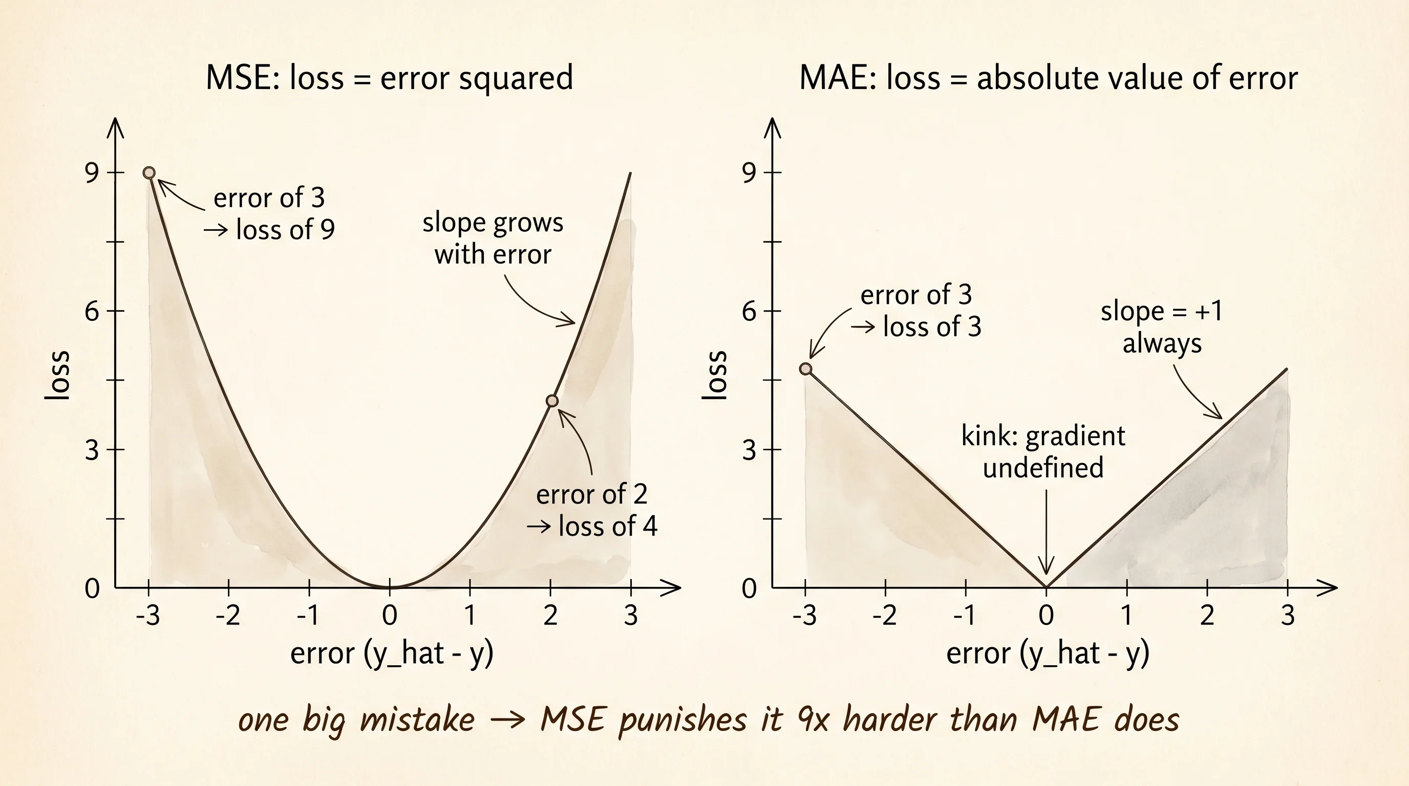
  dL/db = (2/n) * sum (w * x_i + b - y_i)

The error itself enters the MSE gradient. A point off by 4 contributes a term 4 times larger than a point off by 1. Outliers do not just count more — they count quadratically more. That is the whole story of why MSE chases extreme points.

MAE's gradient is meaner to derive because the absolute value has a kink at zero, but it falls out clean. The derivative of |x| is the sign of x — plus 1 on the right of zero, minus 1 on the left, undefined at zero itself. Pick the convention that the gradient at zero is zero and move on.

MAE = (1/n) * sum |w * x_i + b - y_i|
  dL/dw = (1/n) * sum sign(w * x_i + b - y_i) * x_i
  dL/db = (1/n) * sum sign(w * x_i + b - y_i)

Now only the sign of the residual enters the gradient. A point off by 4 contributes the same magnitude as a point off by 0.4. The biggest, ugliest outlier in the dataset pulls the gradient with magnitude 1, no harder than any other point. That is the whole story of why MAE ignores outliers.

Build a small LinearModel with two dials and a forward pass. Wrap the gradients in functions that take the model and the data and return the two slopes. A train function loops the gradient step for a fixed number of epochs.

import random
 
 
class LinearModel:
    def __init__(self, w=0.0, b=0.0):
        self.w = w
        self.b = b
 
    def forward(self, x):
        return self.w * x + self.b
 
 
def mse_gradients(model, data):
    n = len(data)
    grad_w = 0.0
    grad_b = 0.0
    for x, y in data:
        error = model.forward(x) - y
        grad_w += error * x
        grad_b += error
    return (2.0 / n) * grad_w, (2.0 / n) * grad_b
 
 
def sign(value):
    if value > 0.0:
        return 1.0
    if value < 0.0:
        return -1.0
    return 0.0
 
 
def mae_gradients(model, data):
    n = len(data)
    grad_w = 0.0
    grad_b = 0.0
    for x, y in data:
        error = model.forward(x) - y
        s = sign(error)
        grad_w += s * x
        grad_b += s
    return grad_w / n, grad_b / n
 
 
def train(model, loss_fn, gradient_fn, data, lr, epochs):
    for _ in range(epochs):
        grad_w, grad_b = gradient_fn(model, data)
        model.w -= lr * grad_w
        model.b -= lr * grad_b
    return loss_fn(model, data)

Generate 40 noisy points along the true line w = 1.5, b = 0.5 and fit a model with each loss. The function below appends a few extreme outliers when called.

def generate_clean_data(n_points, true_w, true_b, noise_std):
    samples = []
    for _ in range(n_points):
        x = random.uniform(-1.0, 1.0)
        y = true_w * x + true_b + random.gauss(0.0, noise_std)
        samples.append((x, y))
    return samples
 
 
def inject_outliers(data, n_outliers, magnitude):
    contaminated = list(data)
    for _ in range(n_outliers):
        x = random.uniform(-1.0, 1.0)
        contaminated.append((x, magnitude))
    return contaminated

Wire it together. Fit four models — MSE on clean data, MAE on clean data, MSE on contaminated data, MAE on contaminated data — and print the slope and intercept each time.

def mse_loss_model(model, data):
    return mse_loss([model.forward(x) for x, _ in data], [y for _, y in data])
 
 
def mae_loss_model(model, data):
    return mae_loss([model.forward(x) for x, _ in data], [y for _, y in data])
 
 
random.seed(7)
 
clean = generate_clean_data(40, true_w=1.5, true_b=0.5, noise_std=0.1)
 
mse_clean = LinearModel()
train(mse_clean, mse_loss_model, mse_gradients, clean, lr=0.05, epochs=2000)
mae_clean = LinearModel()
train(mae_clean, mae_loss_model, mae_gradients, clean, lr=0.05, epochs=2000)
 
contaminated = inject_outliers(clean, n_outliers=3, magnitude=20.0)
 
mse_dirty = LinearModel()
train(mse_dirty, mse_loss_model, mse_gradients, contaminated, lr=0.05, epochs=2000)
mae_dirty = LinearModel()
train(mae_dirty, mae_loss_model, mae_gradients, contaminated, lr=0.05, epochs=2000)
 
print("before outliers:")
print(f"  MSE w = {mse_clean.w:+.4f}, MSE b = {mse_clean.b:+.4f}")
print(f"  MAE w = {mae_clean.w:+.4f}, MAE b = {mae_clean.b:+.4f}")
print("after outliers:")
print(f"  MSE w = {mse_dirty.w:+.4f}, MSE b = {mse_dirty.b:+.4f}")
print(f"  MAE w = {mae_dirty.w:+.4f}, MAE b = {mae_dirty.b:+.4f}")

Run it.

before outliers:
  MSE w = +1.5143, MSE b = +0.5096
  MAE w = +1.5365, MAE b = +0.5000
after outliers:
  MSE w = -1.9752, MSE b = +1.5402
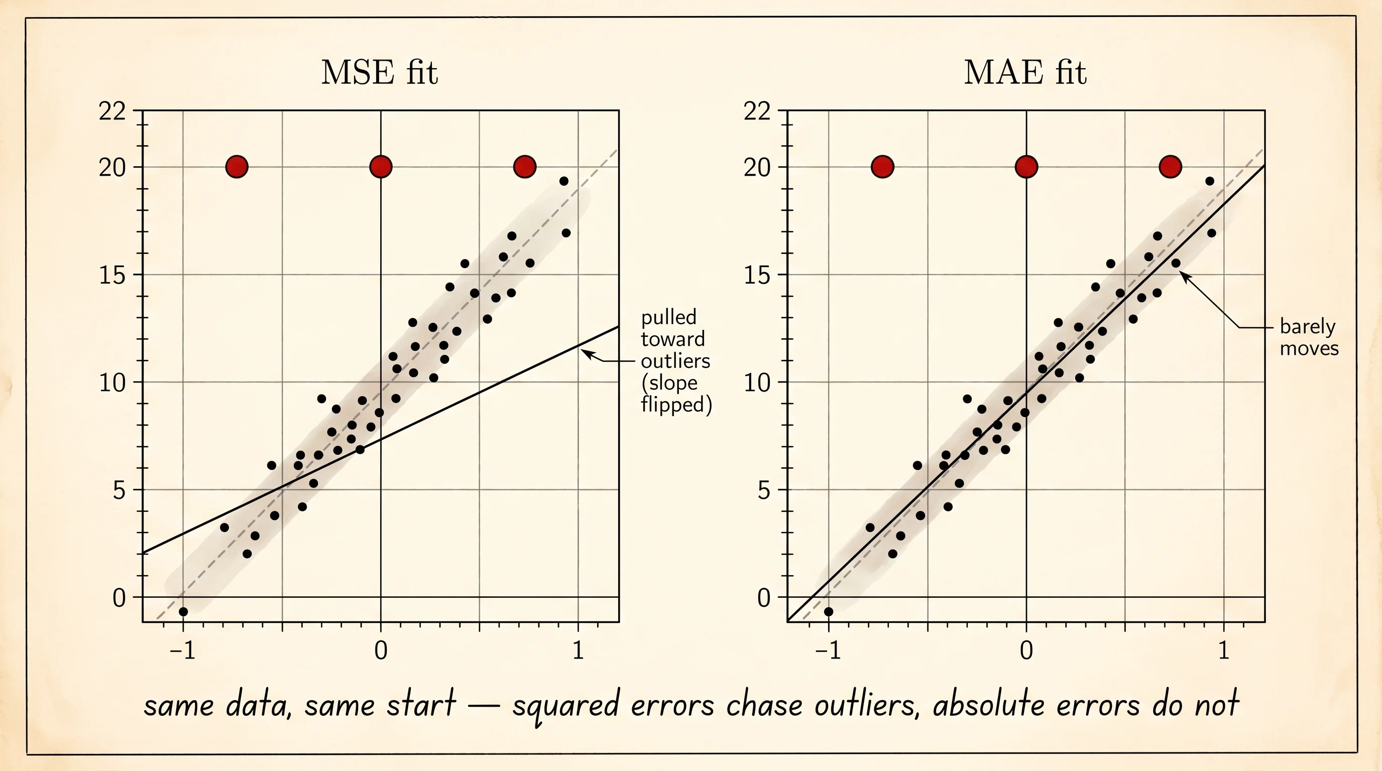
  MAE w = +1.4629, MAE b = +0.4837

Read the four numbers. Before the outliers both losses agree the slope is about 1.5 and the intercept is about 0.5 — they recover the true line up to a hair of noise. After 3 points are dropped at y = 20, the MSE slope swings from +1.51 all the way to −1.97. The line has flipped direction. The fitted MSE line now points the wrong way because 3 huge errors squared dominate the entire average; the gradient says the cheapest move is to tilt the line up toward the outliers and accept being wrong everywhere else. The MAE slope barely moves — from +1.54 to +1.46, a shift of less than 5 percent. Same data. Same starting model. Two coaches, two answers, and the disagreement is the whole point.

A small question. Why did 3 points out of 43 (roughly 7 percent of the data) destroy the MSE fit but leave the MAE fit intact? The answer is in the gradient formulas. Each outlier is off by about 20. The MSE gradient term for one outlier is proportional to 20 — twenty times the size of a normal residual. Three of those swamp the contributions of the 40 well-behaved points combined. The MAE gradient term for one outlier is proportional to sign(20), which is just 1 — exactly the same as the term for a residual of 0.1. The 40 well-behaved points still outvote the 3 outliers because the count is what matters, not the size.

MSE chases outliers. MAE has a kink at zero. You want the smoothness of MSE near the answer with the robustness of MAE at the extremes.