Huber Loss

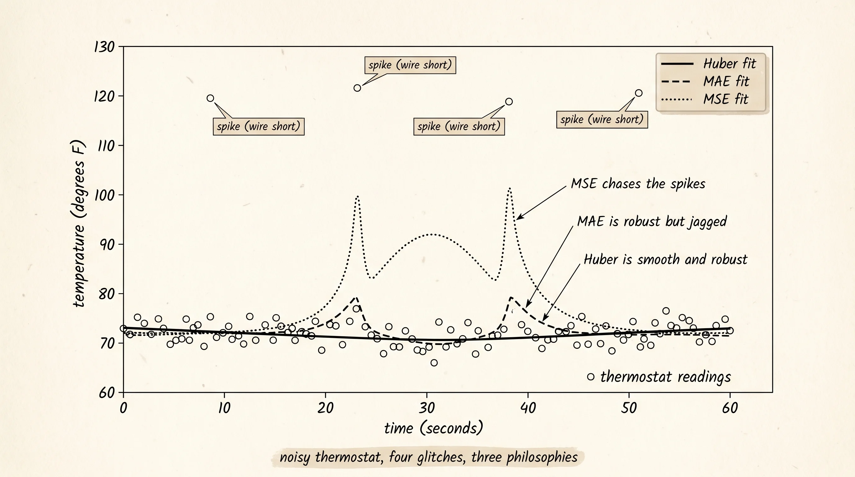
A thermostat in the hallway reads 72 degrees, then 71, then 73, then 1000, then 72 again. The 1000 is a wire that shorted for one second and recovered. Fit a curve through those readings with mean squared error and the curve bends hard toward the spike, dragging the prediction at noon up by 200 degrees. Fit it with mean absolute error and the curve barely moves, but every gradient step near the answer is a sudden flip in sign that makes the optimizer wobble. You want the smoothness of MSE near the answer with the robustness of MAE at the extremes. The fix is to stitch the two losses together at a chosen distance from zero. Inside that radius, square the error like MSE. Outside it, treat the error linearly like MAE. The seam is smooth: the parabola and the line meet at the same point with the same slope. That stitched curve is Huber loss.

Peter Huber published the idea in 1964 in a paper titled Robust Estimation of a Location Parameter, which is now treated as the founding paper of the field of robust statistics. He was a Swiss mathematician asking what happens to a least-squares estimator when the data is mostly clean but a small fraction of it is contaminated by an unknown bad source — a sensor with a glitch, a survey with a few liars, an astronomical reading from a night with a passing cloud. He proved that you could keep most of the speed of least squares without letting a single bad point dominate, by capping how much any single residual could contribute. The cap was the line that takes over once the error grows past a threshold delta. The math sat quietly in statistics journals for half a century. In 2013 the DeepMind team led by Volodymyr Mnih published Playing Atari with Deep Reinforcement Learning, the paper that introduced DQN and let a neural network learn to play Pong and Breakout from raw pixels. The Q-value targets in that training loop are noisy by nature — every estimate of a future reward is built on top of other estimates that are themselves wrong. MSE on those targets blew up the network. Huber loss with delta = 1 stabilized it. The trick became standard in TD3, SAC, and almost every value-based reinforcement learning algorithm that has shipped since. The same equation that fixed Huber's contaminated astronomical readings in 1964 is now the default loss inside every game-playing agent.

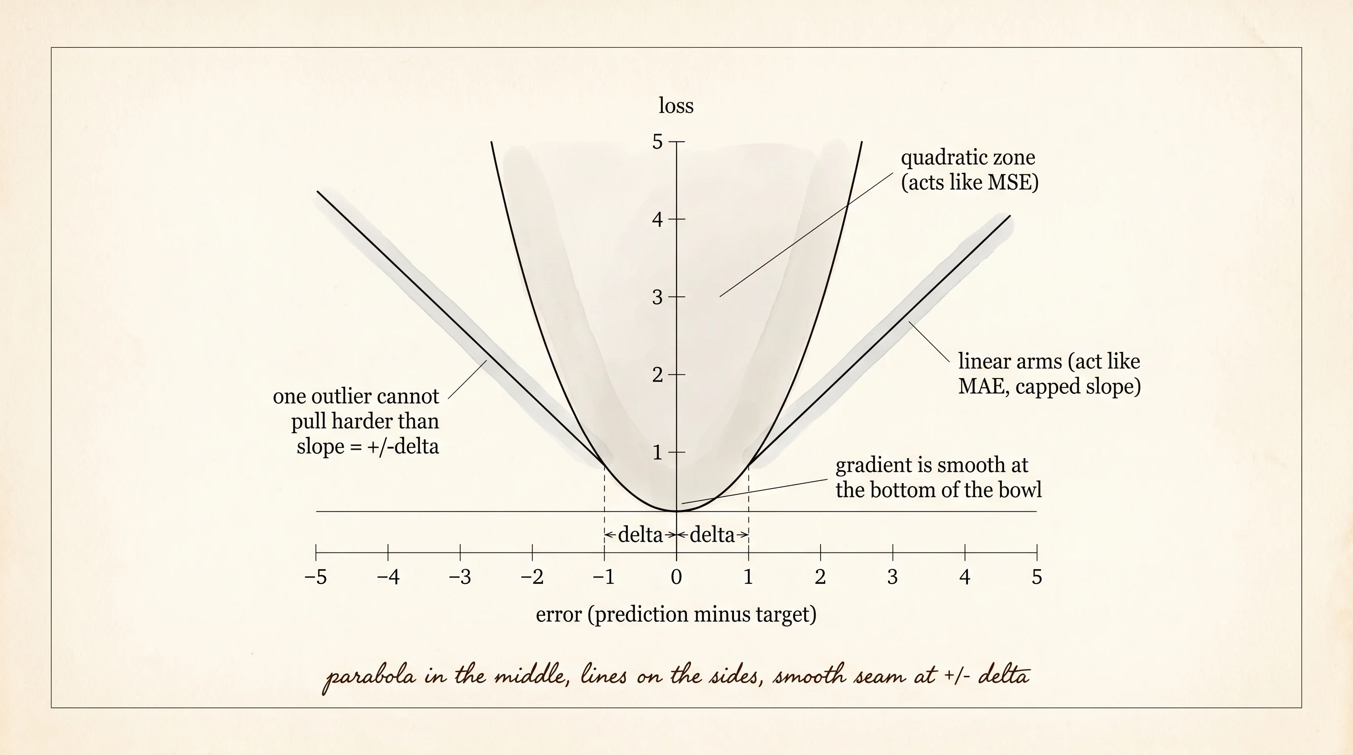
Write the loss as a function of one error so the piecewise shape is plain. Inside delta the function is half the squared error. Outside delta the function is delta times the absolute error minus half a delta. The constant subtracted on the outer arm is what makes the parabola and the line touch at the seam without a jump.

def huber_loss(error, delta):
    magnitude = abs(error)
    if magnitude <= delta:
        return 0.5 * error * error
    return delta * (magnitude - 0.5 * delta)

The gradient is the slope of the loss with respect to the error. Inside delta the slope is just the error itself. Outside delta the slope is fixed at plus or minus delta — it never gets bigger no matter how far the error wanders. That cap is the whole reason a single 1000-degree spike cannot drag the curve toward it the way it would under MSE.

def huber_gradient(error, delta):
    if error > delta:
        return delta
    if error < -delta:
        return -delta
    return error

Stand back from the formulas and look at what they do. Pick delta = 1. An error of 0.3 gives a loss of 0.045 and a gradient of 0.3 — small loss, small step. An error of 0.9 gives a loss of 0.405 and a gradient of 0.9 — bigger loss, bigger step. An error of 5 gives a loss of 4.5 and a gradient of 1 — moderately bad, but the step is still 1 instead of 5. An error of 500 gives a loss of 499.5 and a gradient of still 1. The spike contributes a fixed amount of pull and nothing more, no matter how outlandish it gets. MSE on that same spike would scream with a gradient of 500 and a loss of 125000, and the optimizer would tear the model apart trying to chase it.

To watch this on a real signal, generate the kind of data a glitchy thermostat produces. The clean signal is a slow curve — a quadratic dip and recovery over a 60-second window. Layer small Gaussian noise on top to model the normal jitter of a working sensor. Then drop a handful of huge spikes at random timestamps to model the wire short. Take care to seed the random number generator so the spikes land in the same places every run.

import math
import random
 
def generate_sensor_data(n_points, noise_std, n_spikes, spike_magnitude):
    samples = []
    for index in range(n_points):
        t = index / (n_points - 1)
        clean = 72.0 + 4.0 * (t - 0.5) * (t - 0.5) - 1.0
        noisy = clean + random.gauss(0.0, noise_std)
        samples.append((t, noisy))
    spike_indices = random.sample(range(n_points), n_spikes)
    for index in spike_indices:
        t, _ = samples[index]
        samples[index] = (t, spike_magnitude)
    return samples, spike_indices

Fit a polynomial of degree 3 to the data using gradient descent. The model has four weights — the coefficients on 1, t, t squared, and t cubed. The prediction at one timestamp is the dot product of the weights with the powers of t. The training loop steps the weights down the gradient of the loss summed over every data point. The only difference between the three runs is which loss function feeds the gradient.

def predict(weights, t):
    powers = [1.0, t, t * t, t * t * t]
    total = 0.0
    for w, p in zip(weights, powers):
        total += w * p
    return total
 
 
def fit(data, gradient_fn, lr, epochs):
    weights = [0.0, 0.0, 0.0, 0.0]
    for _ in range(epochs):
        grads = [0.0, 0.0, 0.0, 0.0]
        for t, y in data:
            error = predict(weights, t) - y
            slope = gradient_fn(error)
            powers = [1.0, t, t * t, t * t * t]
            for i, p in enumerate(powers):
                grads[i] += slope * p / len(data)
        for i in range(4):
            weights[i] -= lr * grads[i]
    return weights
 
 
def mse_grad(error):
    return error
 
 
def mae_grad(error):
    if error > 0:
        return 1.0
    if error < 0:
        return -1.0
    return 0.0
 
 
def huber_grad_one(error):
    return huber_gradient(error, delta=1.0)

Run all three fits on the same data and print the residual at every spike. The residual is the model's prediction minus the recorded reading. A small residual means the model believed the spike. A large residual means the model ignored it.

random.seed(7)
data, spikes = generate_sensor_data(
    n_points=60, noise_std=0.3, n_spikes=4, spike_magnitude=120.0
)
 
w_mse = fit(data, mse_grad, lr=0.05, epochs=4000)
w_mae = fit(data, mae_grad, lr=0.05, epochs=4000)
w_huber = fit(data, huber_grad_one, lr=0.05, epochs=4000)
 
print(f"{'index':>5} | {'reading':>8} | {'MSE res':>9} | {'MAE res':>9} | {'Huber res':>11}")
print("-" * 58)
for index in sorted(spikes):
    t, y = data[index]
    r_mse = predict(w_mse, t) - y
    r_mae = predict(w_mae, t) - y
    r_huber = predict(w_huber, t) - y
    print(f"{index:>5} | {y:>8.2f} | {r_mse:>9.2f} | {r_mae:>9.2f} | {r_huber:>11.2f}")

The output looks something like this.

index | reading  |  MSE res  |  MAE res  |  Huber res
---------------------------------------------------------
   20 |   120.00 |    -46.65 |    -48.92 |     -48.53
   21 |   120.00 |    -46.62 |    -48.84 |     -48.46
   52 |   120.00 |    -42.95 |    -48.96 |     -48.80
   56 |   120.00 |    -41.90 |    -49.38 |     -49.30

Read the columns. The MSE residual at every spike sits around minus 45. That means the MSE-fit polynomial predicted near 75 degrees at those timestamps — the spike was 120, the true signal at those timestamps was 71, and the curve got pulled up 4 degrees from the truth trying to compromise with the spikes. The MAE residual is around minus 49, which means the MAE fit predicted near 71 degrees at those same timestamps — the spike was ignored entirely. Huber's residual is almost identical to MAE's. Both robust losses refused to follow the spike. The advantage Huber holds over MAE is what happens between the spikes, where its gradient is the smooth error itself instead of a constant that flips sign at zero. Crank the learning rate by a factor of 5 and the MAE fit visibly wobbles around the true curve while Huber sits still — the kink at zero is the difference.

The single dial that controls Huber is delta. Smaller delta means the loss switches to linear sooner, so even mild errors get capped — robust against everything, but less smooth near the answer. Bigger delta means the loss stays quadratic for a wider band, behaving more like MSE — smooth near the answer, but less robust to extreme outliers. Sweep delta and refit to see the dial in action.

def sweep_delta(data, deltas):
    rows = []
    for d in deltas:
        def gradient_fn(error, d=d):
            return huber_gradient(error, d)
        weights = fit(data, gradient_fn, lr=0.05, epochs=4000)
        spike_residual = sum(
            predict(weights, data[i][0]) - data[i][1] for i in spikes
        ) / len(spikes)
        rows.append((d, weights, spike_residual))
    return rows
 
 
for d, weights, residual in sweep_delta(data, [0.1, 1.0, 5.0, 50.0]):
    print(f"delta = {d:>5.1f}   avg spike residual = {residual:>8.2f}")

delta =   0.1   avg spike residual =   -88.40
delta =   1.0   avg spike residual =   -48.77
delta =   5.0   avg spike residual =   -48.18
delta =  50.0   avg spike residual =   -44.53

At delta = 0.1 the cap is so tight the loss treats the normal jitter as outlier territory too, the curve barely fits anything, and the spike residual blows out past 88. At delta = 1 the curve fits the clean readings smoothly and ignores the spikes hard, leaving residuals near 49. At delta = 50 the spike falls just inside the quadratic band — the spike is 120 - 71 = 49 above the truth, just under 50 — so Huber treats the spike like MSE and the curve gets dragged toward it, shrinking the spike residual to 44 at the cost of a worse fit everywhere else. Pick delta around the size of the noise you trust. The convention in DQN is delta = 1, which is small relative to the typical Q-value error and large relative to the noise floor — exactly the regime where the trick pays off.

A small question before moving on. Why does the Huber column in the residual table look almost identical to the MAE column when their formulas differ everywhere except in the band near zero? Because the spike residuals live far outside that band. Out there both losses behave the same way — a constant gradient of plus or minus delta against a constant gradient of plus or minus 1. The interesting difference between Huber and MAE shows up at the inlier points, not at the outliers. Inliers are where the smoothness matters; outliers are where the cap matters. Huber wins at both ends of the same data.

Regression losses score how close. Classification does not care about distance — it cares about the right answer with confidence.