Hinge Loss and Margins

Regression losses score how close. Classification doesn't care about distance — it cares about the right answer with confidence. Walk into a powerlifting meet and watch the head judge. The lifter racks 405 pounds, drives it off his chest, the bar drifts up, the elbows almost lock — and then he racks it. Three white lights? No. Three red lights. A barely-completed rep is a no-lift. The judge does not reward "almost." The judge wants the elbows locked out hard, the bar held still, no doubt. Hinge loss is that judge wearing a math hat. Predicting on the right side of zero isn't enough. You have to predict on the right side of zero by at least 1, and only then does the loss go quiet.

The idea came out of Moscow. In 1963 Vladimir Vapnik and Alexey Chervonenkis published a paper in Russian on what they called the optimal separating hyperplane — pick the boundary between two classes that sits as far from the closest training points as possible. The West did not notice for 20 years. The Soviet pattern-recognition community kept refining it through the 1970s and 1980s while American statisticians chased neural networks and decision trees. In 1995 Corinna Cortes and Vapnik (now at Bell Labs) published Support-Vector Networks, which extended the original idea to data that does not separate cleanly by allowing some points to violate the margin for a price. The price was hinge loss. The paper detonated. Through the 2000s the support vector machine ate every machine-learning competition that involved fewer than 100,000 training examples. Faces, handwritten digits, protein structures, spam — SVMs won them all. Then in 2012 Alex Krizhevsky's deep convolutional network beat the entire SVM field on ImageNet by a margin nobody had ever seen, and the SVM era ended overnight. The loss function did not die. Hinge loss is still the standard loss whenever you want a hard-margin classifier without probability estimates, and the geometric idea behind it — find the boundary with the widest gap — is still the cleanest mental model for what a binary classifier is doing.

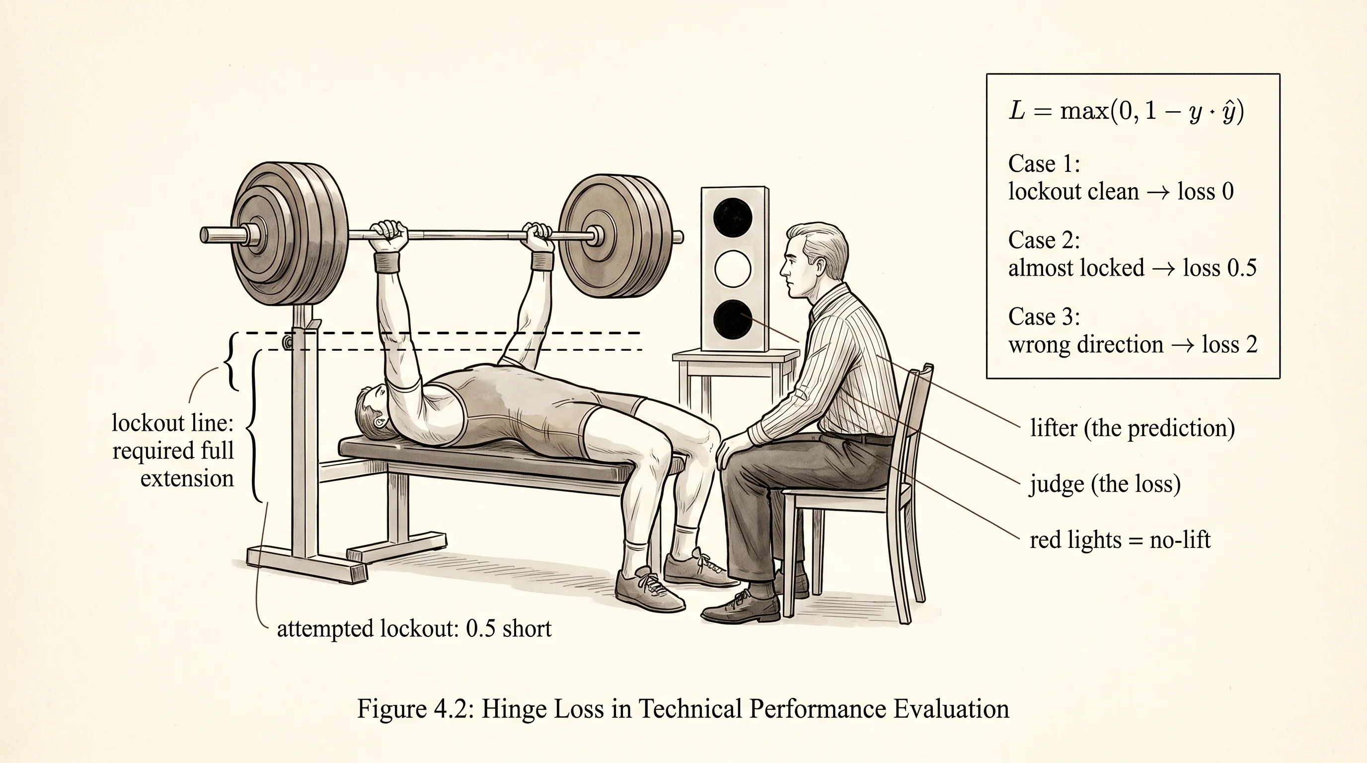
The math is one line. Label the two classes +1 and -1. Let y_hat be the raw decision value the classifier emits — not a probability, just a number whose sign picks the class. Hinge loss takes one prediction and one label and returns max(0, 1 - y * y_hat).

def hinge_loss(y_true, y_pred):
    margin = 1.0 - y_true * y_pred
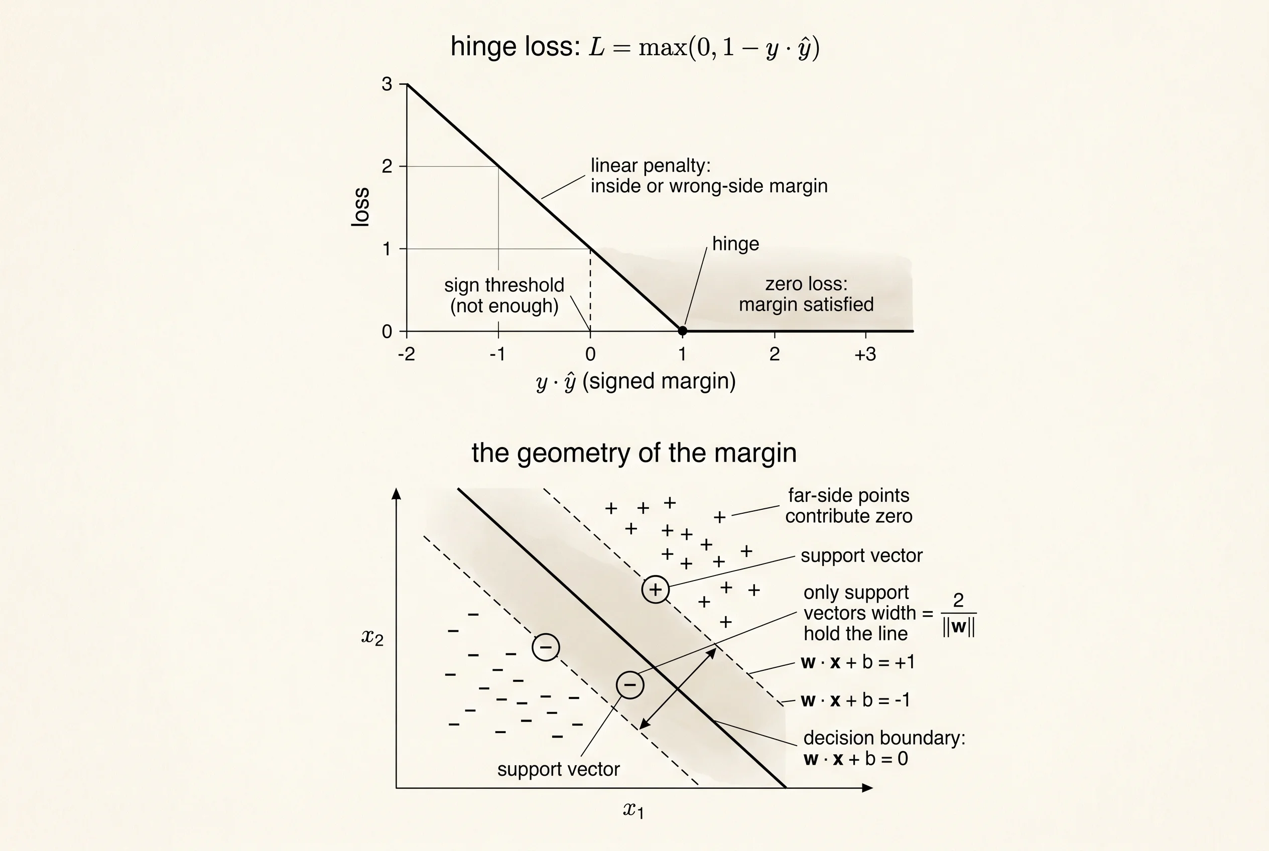
    return margin if margin > 0.0 else 0.0

Walk three cases through it. A point with label +1 and prediction +2: the product is +2, the margin is 1 - 2 = -1, the loss is 0. The judge nods. A point with label +1 and prediction +0.5: the product is +0.5, the margin is 1 - 0.5 = +0.5, the loss is 0.5. The lift went up but the elbows did not lock; the judge docks half a point. A point with label +1 and prediction -1: the product is -1, the margin is 1 - (-1) = +2, the loss is 2. Wrong side of the bar. Two-point penalty. The size of the penalty grows linearly the further you fail in the wrong direction, and the penalty stops dead at the moment the prediction crosses the +1 line on the right side.

That flat zero region on the right side is the unique fingerprint of hinge loss. Squared error keeps pushing forever — even a perfect prediction has zero gradient only at the exact point of equality. Hinge gives a free pass to every prediction that is confidently correct. Confidently means by at least 1, which is the unit chosen by convention; the actual width depends on the scale of the weights, which is what regularization is for.

The gradient is the next line. Differentiate 1 - y * y_hat with respect to the weights. The decision value y_hat = w . x + b, so the derivative of y_hat with respect to w_i is x_i, and the derivative of 1 - y * y_hat is -y * x_i. That is the active gradient. When the example is outside the margin and the loss is zero, the gradient is also zero — the hinge has flattened to a horizontal line and there is no slope to descend. That gives a clean piecewise rule.

def hinge_gradient(y_true, y_pred, x):
    if 1.0 - y_true * y_pred <= 0.0:
        return [0.0] * len(x), 0.0
    weight_grad = [-y_true * xi for xi in x]
    bias_grad = -y_true
    return weight_grad, bias_grad

Two things follow from this rule. First, training only updates the weights using the points that are currently inside the margin or on the wrong side. The deep-interior correctly-classified points are silent observers. Second, as the boundary settles into its final shape, fewer points sit inside the margin, fewer gradients fire, and the effective batch size shrinks. The points that survive as gradient contributors all the way to the end are the support vectors. They are the only data the final boundary depends on. Throw away every other point and retrain — you get the exact same line.

The classifier itself is the same one-neuron object you have already built, minus the activation. Pure linear: a weight per feature, a bias, and a decision function that returns the raw w . x + b. The label prediction is the sign of that value.

import math
import random
 
class LinearClassifier:
    def __init__(self, n_features):
        scale = 1.0 / math.sqrt(n_features)
        self.weights = [random.gauss(0.0, scale) for _ in range(n_features)]
        self.bias = 0.0
 
    def decision(self, x):
        total = self.bias
        for w, xi in zip(self.weights, x):
            total += w * xi
        return total
 
    def predict(self, x):
        return 1.0 if self.decision(x) >= 0.0 else -1.0

Now write the function that picks out the support vectors. A support vector is any point where the hinge loss is non-zero, which is exactly the condition 0 < 1 - y * (w . x + b). Any point that satisfies it sits inside the margin band or on the wrong side of the boundary.

def identify_support_vectors(classifier, data):
    return [
        (x, y) for x, y in data if 1.0 - y * classifier.decision(x) > 0.0
    ]

To watch the boundary settle you need a way to see it. Print the 2D plane as a grid where each cell is colored by which side of the boundary it sits on, with a third color for the margin band. Three glyphs: . for the positive side beyond the margin, , for the negative side beyond the margin, : for the band itself. Then overlay every data point: + for label +1, - for label -1, and @ for any point that is currently a support vector.

def print_decision_boundary(classifier, data, grid_size, support_vectors=None):
    sv_set = {(round(x[0], 6), round(x[1], 6)) for x, _ in (support_vectors or [])}
    rows = []
    for r in range(grid_size):
        y_coord = 3.0 - 6.0 * r / (grid_size - 1)
        line = []
        for c in range(grid_size):
            x_coord = -3.0 + 6.0 * c / (grid_size - 1)
            score = classifier.decision([x_coord, y_coord])
            if abs(score) < 1.0:
                line.append(":")
            elif score >= 0.0:
                line.append(".")
            else:
                line.append(",")
        rows.append(line)
    for x, y in data:
        col = int(round((x[0] + 3.0) / 6.0 * (grid_size - 1)))
        row = int(round((3.0 - x[1]) / 6.0 * (grid_size - 1)))
        if 0 <= row < grid_size and 0 <= col < grid_size:
            key = (round(x[0], 6), round(x[1], 6))
            rows[row][col] = "@" if key in sv_set else ("+" if y > 0.0 else "-")
    return "\n".join("".join(line) for line in rows)

Wire it together. Generate 60 noisy two-class points along a true boundary, count the support vectors at random initialization, train for 400 epochs of plain gradient descent on the average hinge loss, count the support vectors again, and print the boundary at both ends of training.

random.seed(7)
 
data = generate_two_class_data(n_per_class=30, true_w=[1.0, -0.6], true_b=0.4, noise=0.5)
classifier = LinearClassifier(n_features=2)
 
initial_sv = identify_support_vectors(classifier, data)
print(f"support vectors before training: {len(initial_sv)} of {len(data)}")
 
train(classifier, data, learning_rate=0.05, n_epochs=400, reg_strength=0.01)
 
final_sv = identify_support_vectors(classifier, data)
print(f"support vectors after training:  {len(final_sv)} of {len(data)}")

Run it and read the two numbers.

support vectors before training: 34 of 60
initial mean hinge loss: 0.5306
 
decision boundary at random init:
,,,::::::::::@:..+...
,,,::::::::::@:..+...
,,,::::@:::@:::......
,,,:::::@::::::......
,,,,:::::::@:::..+...
,-,,::::@:::::::+....
,-,,::::::::::::++...
,,,,::::@:::::::.....
,,,,-:::::@:::::.....
,,,,:::@:::::::@.....
,-,-,@:::@::::::.....
-,-,,:::::::@:@::....
-,,,,:@:@:::@::::....
,,-,,@:::::@:@:::....
,,,,,::::@:::::@:++..
,,,--::@:::::::::....
,-,,,,:@:::::::::....
-,,,-,@::::@@::::@...
,-,-,,::::::::::::...
,-,,,,:@:::@::@:::...
,,,,,,::::::::::::...
 
support vectors after training:  15 of 60
final mean hinge loss:   0.1480
learned w = (+1.638, -1.006), b = +0.545
 
decision boundary after training (@ = support vector):
,,,,,,,,,,,,,@:::@...
,,,,,,,,,,,,,@:::+...
,,,,,,,-,,,-::::.....
,,,,,,,,-,,,::::.....
,,,,,,,,,,,@:::..+...
,-,,,,,,-,::::..+....
,-,,,,,,,,::::..++...
,,,,,,,,-::::........
,,,,-,,,,:@::........
,,,,,,,@::::...+.....
,-,-,-,::@:..........
-,-,,,,::::.+.+......
-,,,,,-:@:..+........
,,-,,@::::.+.+.......
,,,,,::::+.....+.++..
,,,--::@.............
,-,,:::@.............
-,,:@:@....++....+...
,-:@:::..............
,-::::.+...+..+......
,::::................

Read the count first. Before training, 34 of 60 points are support vectors — more than half the dataset is inside the margin or on the wrong side, because the random initial line is wandering through the middle of both classes. After training, 15 of 60. The line has rotated to its proper angle, the margin band has shifted to sit between the two clouds, and most of the data is now safely outside the band on its own side. The 15 points that remain are the points the boundary actually depends on. Some of them are on the wrong side because the data is noisy and not perfectly separable; some sit inside the band because they are honestly close to the line. Those are the lifters whose grades are still being read.

Read the picture next. The first grid has the colon-shaded margin band running diagonally from the top-right down through the middle, with @ symbols scattered on both sides of it — 34 unhappy points. The second grid has the same band but tilted to the proper angle, with the + cluster pushed safely into the upper-right region and the - cluster into the lower-left. The handful of @ symbols that remain trace the edges of the band and a few stragglers on the wrong side of the line. That is the geometric meaning of "support vector" — the points sitting on or near the gap, the ones whose presence physically holds the line in place.

A small question. If a confidently-correct point contributes zero loss and zero gradient, why does anyone train on the whole dataset instead of just the support vectors? You don't know which points are support vectors until after training. The set is defined by where the final boundary lands, not by the data on its own. You discover them by running the algorithm — and during training the membership of the set keeps changing as the line moves. A point that was a support vector at epoch 5 may have drifted safely outside the margin by epoch 200, replaced by a different point that fell inside.

Hinge loss separates classes. It doesn't tell you the probability that a point is in a class.