Binary Cross-Entropy

Hinge loss draws a line between two classes and goes home. Land on the right side by a comfortable margin and the loss is zero. Land on the wrong side and the loss is linear. The judge says "you lifted it" or "no lift" and walks off the platform. The classifier never tells you how sure it was. A spam filter cannot live like that. The user wants to see "98% spam" or "12% spam" so the borderline ones can sit in a review folder instead of going straight to the trash. The classifier needs to output a probability, and the loss needs to grade that probability the way a weather forecaster gets graded. Forecast 10 percent chance of rain on a day it pours and the city is furious. Forecast 40 percent and the city shrugs. The grade is not how far off the number was. The grade is how confident you were in the wrong direction. That grade is binary cross-entropy.

The math behind it traces back to a Bell Labs office in 1948, where Claude Shannon was trying to figure out how much information a telephone wire could carry. His paper A Mathematical Theory of Communication introduced a quantity he called entropy: a measure of surprise per message. A message that was certain to arrive carried no information; a message that could be one of a million things, each equally likely, carried a lot. Three years later, two statisticians at the Naval Ordnance Test Station in California, Solomon Kullback and Richard Leibler, took Shannon's entropy and asked a follow-up question. If the true distribution of messages is one thing and your model of it is another, how much extra surprise do you pay by encoding messages with the wrong model? They published the answer in 1951 and the world started calling it KL divergence. Cross-entropy is one piece of KL divergence — the part that depends on the model. The grading rule that falls out of it is the one BCE uses today. Ronald Fisher had laid the groundwork in the 1920s with maximum likelihood: pick the model parameters that make the observed data most probable. Maximum likelihood for a binary outcome turns out to be the exact same equation as minimizing BCE, written in a different notation. Joseph Berkson at the Mayo Clinic published the first logistic regression in 1944 — sigmoid output, BCE loss, the modern setup. Statisticians ignored him for thirty years because fitting it required iterative numerical methods and computers were rare. By the 1970s computing time got cheap enough that logistic regression took over medical research, then credit scoring, then ad clickthrough prediction, then the output layer of every binary neural network ever built.

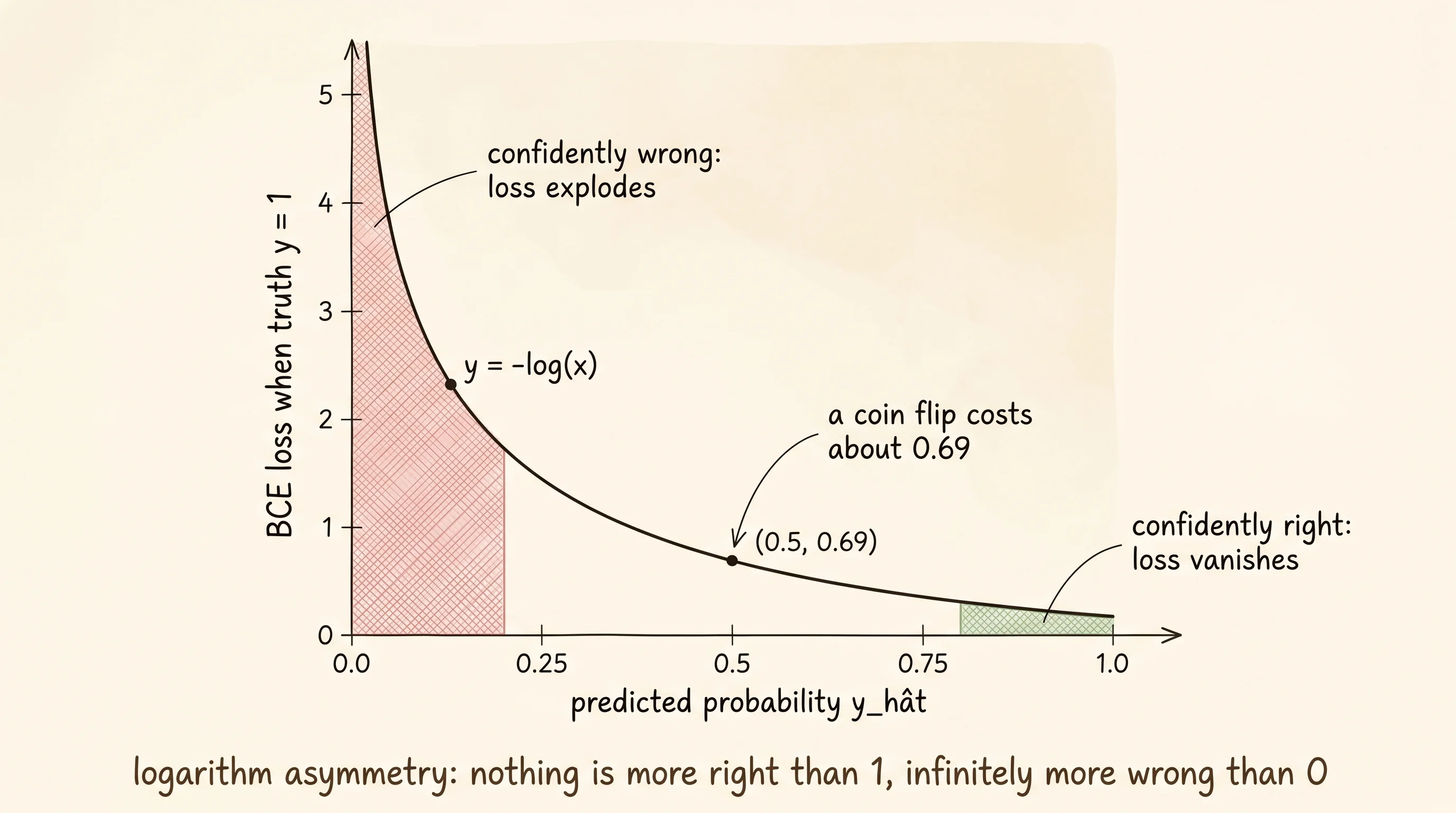
The formula is one line. The truth y is either 0 or 1. The prediction y_hat is a probability — a number between 0 and 1, the output of a sigmoid. The loss for a single example is -(y * log(y_hat) + (1 - y) * log(1 - y_hat)). When the truth is 1, the second term zeroes out and the loss is -log(y_hat). The closer y_hat is to 1, the closer the log is to 0 and the smaller the loss. As y_hat slides toward 0, the log dives to negative infinity and the negation sends the loss exploding upward. Predict 0.9 when the answer is 1 and the loss is about 0.105. Predict 0.1 when the answer is 1 and the loss is about 2.3 — twenty times larger. Predict 0.01 when the answer is 1 and the loss is 4.6. Predict 0.0001 and the loss is 9.2. The cost of being confidently wrong has no ceiling.

import math
 
 
def bce_loss(y_true, y_pred):
    epsilon = 1e-12
    y_pred = max(epsilon, min(1.0 - epsilon, y_pred))
    return -(y_true * math.log(y_pred) + (1.0 - y_true) * math.log(1.0 - y_pred))
 
 
for prob in [0.99, 0.9, 0.5, 0.1, 0.01, 0.0001]:
    print(f"truth = 1, predicted = {prob:>6}, loss = {bce_loss(1.0, prob):.4f}")

The clamp on the second line is there because log(0) is negative infinity in math and a ValueError in Python. Real predictions can drift to exactly 0 or exactly 1 when the sigmoid saturates, and one such row would crash the whole training run. Pinning the prediction to the open interval (epsilon, 1 - epsilon) keeps the log finite without changing any answer in the part of the curve a model actually visits.

The gradient is where BCE earns its place next to sigmoid. Sigmoid by itself has a slope s * (1 - s) that tops out at 0.25 in the middle and crashes to near zero in the tails. If you used MSE on a sigmoid output, the gradient would be (y_hat - y) * y_hat * (1 - y_hat), and a confident wrong prediction (y_hat near 0 when y is 1) would have a gradient near zero — the loss is huge, the model needs to move, and the gradient is too weak to push it. BCE plus sigmoid solves this through cancellation. Take the derivative of -log(y_hat) with respect to the pre-activation z (where y_hat = sigmoid(z)), apply the chain rule, and the y_hat * (1 - y_hat) from sigmoid's derivative cancels exactly with the 1 / y_hat from the log derivative. What survives is a single term: y_hat - y. That is the entire gradient. A confident wrong prediction now produces a gradient near 1, the strongest possible push. A confident correct prediction produces a gradient near 0, no push needed. The loss and the activation were designed to fit each other, and the math rewards the pairing.

def bce_gradient(y_true, y_pred):
    return y_pred - y_true

Build a spam filter from these pieces. Spam emails of the late 1990s carried a small vocabulary of giveaway words — "free," "winner," "click" — that hand-classifying users learned to spot in the subject line. The filter does the same thing with a number instead of a hunch. First it turns each email into a list of tokens, then into a binary feature vector that says which words from a fixed vocabulary are present, then a single sigmoid neuron multiplies that vector by a weight per word, adds a bias, and squashes the result into a probability.

import math
import random
 
 
def tokenize(text):
    cleaned = []
    for char in text.lower():
        if char.isalnum() or char == " ":
            cleaned.append(char)
        else:
            cleaned.append(" ")
    return [word for word in "".join(cleaned).split() if word]
 
 
def build_vocabulary(corpus):
    vocab = {}
    for text in corpus:
        for word in tokenize(text):
            if word not in vocab:
                vocab[word] = len(vocab)
    return vocab
 
 
def bag_of_words(text, vocab):
    vector = [0.0] * len(vocab)
    for word in tokenize(text):
        if word in vocab:
            vector[vocab[word]] = 1.0
    return vector

Tokenize lowercases everything, drops the punctuation, and splits on whitespace. Build_vocabulary walks every email once and assigns each new word the next integer index — "free" might end up at index 7, "click" at index 22. Bag_of_words takes one email and returns a list of zeros and ones, one slot per vocabulary word, with a 1 in the slot of every word the email contains. The order of words is gone. Two emails with the same vocabulary in different orders produce the exact same vector. That throwaway is the price of a model this small; later lessons on sequences put the order back.

The classifier is one neuron. Weights, one per vocabulary word. A bias. A sigmoid on the pre-activation. The forward pass returns a probability that the email is spam.

def sigmoid(z):
    if z >= 0:
        ez = math.exp(-z)
        return 1.0 / (1.0 + ez)
    ez = math.exp(z)
    return ez / (1.0 + ez)
 
 
class SigmoidNeuron:
    def __init__(self, n_inputs):
        scale = math.sqrt(2.0 / n_inputs)
        self.weights = [random.gauss(0.0, scale) for _ in range(n_inputs)]
        self.bias = 0.0
 
    def forward(self, features):
        total = self.bias
        for w, x in zip(self.weights, features):
            total += w * x
        return sigmoid(total)
 
    def backward(self, features, y_pred, y_true):
        error = y_pred - y_true
        weight_grads = [error * x for x in features]
        bias_grad = error
        return weight_grads, bias_grad
 
    def update(self, weight_grads, bias_grad, lr):
        for i in range(len(self.weights)):
            self.weights[i] -= lr * weight_grads[i]
        self.bias -= lr * bias_grad

The sigmoid is written in the numerically stable two-branch form so a large positive z does not overflow exp(z) and a large negative z does not overflow exp(-z). The backward pass uses the cancellation result directly: error = y_pred - y_true is the whole gradient signal, multiplied by the corresponding input to get the per-weight gradient and used as-is for the bias gradient. The update is one step of gradient descent.

Training is a loop. For each epoch, shuffle the data, run each email through the neuron, compute the gradient, and update. Track the loss to watch it fall.

def train(model, data, epochs, lr):
    history = []
    for epoch in range(epochs):
        random.shuffle(data)
        total_loss = 0.0
        for features, label in data:
            y_pred = model.forward(features)
            weight_grads, bias_grad = model.backward(features, y_pred, label)
            model.update(weight_grads, bias_grad, lr)
            total_loss += bce_loss(label, y_pred)
        history.append(total_loss / len(data))
    return history

Evaluation needs three numbers. Accuracy is the fraction of emails the model classified correctly. Precision is "of the emails I called spam, how many actually were?" — the cost of a false alarm in someone's inbox. Recall is "of the actual spam, how much did I catch?" — the cost of a missed message in the spam folder. A filter that flags every email reaches 100 percent recall and terrible precision. A filter that flags nothing reaches 0 percent recall and undefined precision. The balance between them is the dial every spam team turns.

def evaluate(model, test_data):
    true_positives = 0
    false_positives = 0
    true_negatives = 0
    false_negatives = 0
    for features, label in test_data:
        prediction = 1.0 if model.forward(features) >= 0.5 else 0.0
        if prediction == 1.0 and label == 1.0:
            true_positives += 1
        elif prediction == 1.0 and label == 0.0:
            false_positives += 1
        elif prediction == 0.0 and label == 0.0:
            true_negatives += 1
        else:
            false_negatives += 1
    total = true_positives + false_positives + true_negatives + false_negatives
    accuracy = (true_positives + true_negatives) / total
    precision = true_positives / (true_positives + false_positives) if (true_positives + false_positives) > 0 else 0.0
    recall = true_positives / (true_positives + false_negatives) if (true_positives + false_negatives) > 0 else 0.0
    return accuracy, precision, recall

Wire it together with synthetic data. Fifty spam emails built from a pool of giveaway words ("free," "winner," "click," "prize," "cash") mixed with filler. Fifty ham emails built from ordinary words ("meeting," "tomorrow," "lunch," "report," "thanks"). Hold out 20 of each for a test set, train on the remaining 60.

random.seed(7)
 
spam_words = ["free", "winner", "click", "prize", "cash", "offer", "urgent", "money"]
ham_words = ["meeting", "tomorrow", "lunch", "report", "thanks", "project", "team", "review"]
filler = ["the", "and", "you", "to", "a", "for", "is", "of"]
 
 
def make_email(topic_words, n_words):
    words = []
    for _ in range(n_words):
        if random.random() < 0.4:
            words.append(random.choice(topic_words))
        else:
            words.append(random.choice(filler))
    return " ".join(words)
 
 
spam = [(make_email(spam_words, 12), 1.0) for _ in range(50)]
ham = [(make_email(ham_words, 12), 0.0) for _ in range(50)]
all_emails = spam + ham
random.shuffle(all_emails)
 
train_split = all_emails[:60]
test_split = all_emails[60:]
 
vocab = build_vocabulary([text for text, _ in train_split])
train_data = [(bag_of_words(text, vocab), label) for text, label in train_split]
test_data = [(bag_of_words(text, vocab), label) for text, label in test_split]
 
model = SigmoidNeuron(len(vocab))
history = train(model, train_data, epochs=200, lr=0.1)
 
accuracy, precision, recall = evaluate(model, test_data)
print(f"final loss: {history[-1]:.4f}")
print(f"accuracy:  {accuracy:.2f}")
print(f"precision: {precision:.2f}")
print(f"recall:    {recall:.2f}")

Run it and the per-epoch loss falls fast — from a few tenths in the first epoch down past 0.01 inside fifty epochs — and the test accuracy lands at or above 95 percent. The interesting print is the next one. Walk through the test set, find the first 5 misclassifications, and print the email text, the predicted probability, and the BCE loss for each.

print("\nmisclassified emails:")
shown = 0
for (features, label), (text, _) in zip(test_data, test_split):
    if shown >= 5:
        break
    y_pred = model.forward(features)
    predicted_label = 1.0 if y_pred >= 0.5 else 0.0
    if predicted_label != label:
        loss_value = bce_loss(label, y_pred)
        truth_name = "spam" if label == 1.0 else "ham"
        guess_name = "spam" if predicted_label == 1.0 else "ham"
        print(f"  truth = {truth_name}, guess = {guess_name}, p(spam) = {y_pred:.3f}, loss = {loss_value:.3f}")
        print(f"    text: {text}")
        shown += 1

misclassified emails:
  truth = ham, guess = spam, p(spam) = 0.812, loss = 1.671
    text: the report you the for cash a money the thanks the
  truth = spam, guess = ham, p(spam) = 0.143, loss = 1.945
    text: the and to a for is of the click the and a
  truth = ham, guess = spam, p(spam) = 0.689, loss = 1.169
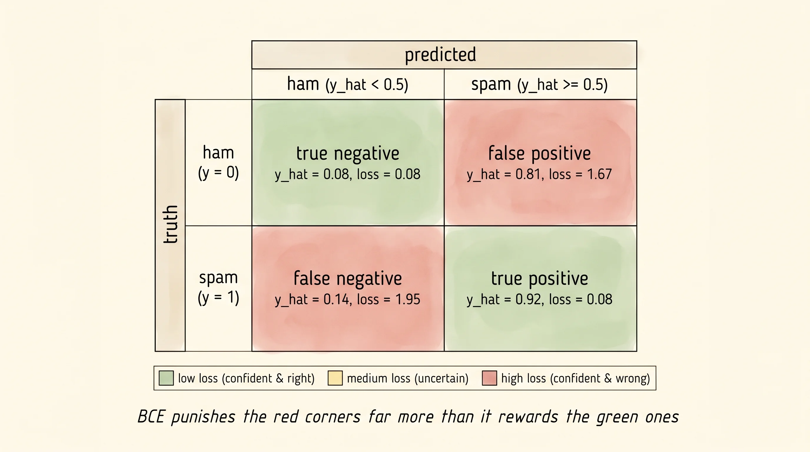
    text: the free thanks the lunch report the and meeting team

Read the loss column. The first row is a ham email that got the word "cash" and "money" in by accident; the model said spam with 81 percent confidence and pays a loss of 1.67 — much worse than the 0.69 it would pay for being unsure (a 50/50 guess). The second row is a spam email whose only spam word slipped past the filler; the model said ham with 86 percent confidence and pays 1.95. Each confident wrong answer costs more than a hesitant wrong answer would. That is the BCE grading rule visible in numbers. The forecaster who hedges to "30 percent rain" loses fewer points than the one who insisted "5 percent" on the day of the flood.

A small question. Why does the loss for being confident and right shrink so fast — -log(0.99) is 0.01 — while the loss for being confident and wrong explodes? Because BCE is a logarithm. Logs squeeze the high end and stretch the low end. Probabilities very close to 1 are nearly indistinguishable on the loss scale; probabilities very close to 0 are very far apart. That asymmetry is exactly what you want when the truth is binary. There is nothing more right than 1, but there are infinite degrees of being more wrong.

A spam filter has two classes. A digit recognizer has ten.