Categorical Cross-Entropy

A multiple-choice question with four bubbles in front of you, A through D. Pick A and you are right. Pick anything else and you are wrong. The teacher who hands back this exam adds one twist: she does not just want your bubble, she wants your confidence. Bubble A with 99% confidence and the answer is A and your loss is almost zero — you knew it, you said it, you are done. Bubble A with 99% confidence and the answer is C and the loss is catastrophic. The grade is no longer "right or wrong." The grade is "how badly did you commit to wrong." That confidence-weighted grade, written in the language of probabilities and logs, is categorical cross-entropy.

The math comes from the same lineage as binary cross-entropy. Claude Shannon at Bell Labs in 1948 wrote down a formula for the surprise carried by a single message — log of one over its probability — and gave the field the word "entropy." Three years later Solomon Kullback and Richard Leibler, two cryptanalysts who had spent the war breaking codes, asked a different question: given two probability distributions, how far apart are they? Their answer, KL divergence, is just the average extra surprise you suffer when you predict with the wrong distribution. R. A. Fisher had been computing the same quantity since the 1920s under the name maximum likelihood, but nobody connected the three threads until the 1950s. Logistic regression and the binary case won first because two classes is the easy version. The N-class generalization sat in textbooks for decades, used by linguists and bird-counting biologists, ignored by mainstream computing — until 2012, when Alex Krizhevsky took a network with categorical cross-entropy on the output and 1000 classes from ImageNet, ran it on two GPUs in his bedroom, and beat the second-place team by a margin so wide the conference paper announcing it changed the field overnight. Every vision and language model since — VGG, ResNet, BERT, GPT-2, GPT-3, GPT-4 — uses the same loss function. The architectures keep changing. The loss has not moved.

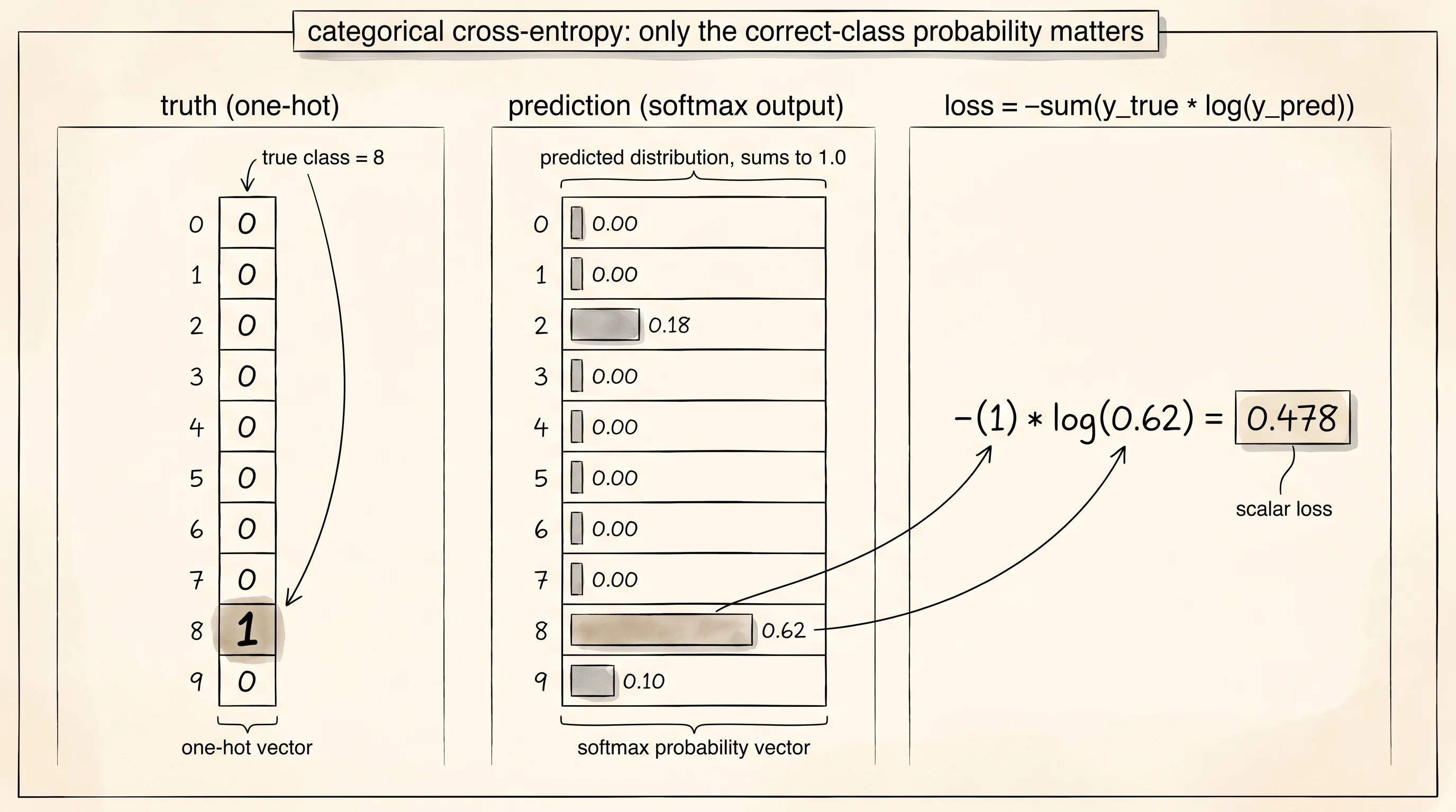
The setup is two vectors. The first vector is the truth, written one-hot — a list of 10 numbers where exactly one entry is 1 and the other 9 are 0. If the right answer is digit 8, the truth vector is [0, 0, 0, 0, 0, 0, 0, 0, 1, 0]. The second vector is the model's prediction — a list of 10 probabilities that add up to 1. The model says "I think it is digit 8 with 0.62 confidence, digit 3 with 0.18, and the rest split between the remaining 8 classes." Categorical cross-entropy compares the two by walking down the list, multiplying each truth entry by the log of the matching prediction entry, summing, and flipping the sign.

import math
 
def categorical_cross_entropy(y_true, y_pred):
    epsilon = 1e-12
    total = 0.0
    for truth, prediction in zip(y_true, y_pred):
        clamped = max(prediction, epsilon)
        total -= truth * math.log(clamped)
    return total

Read the loop. Every term is truth * log(prediction). The truth is 0 for 9 of the 10 classes, so 9 of the 10 terms drop out. Only one term survives — the log of the probability the model assigned to the correct class. If the model said 0.99 for the right class, the loss is -log(0.99), which is 0.01. If the model said 0.01 for the right class, the loss is -log(0.01), which is 4.6. If the model said 0.0001, the loss is 9.2. The penalty grows without bound the more confidently wrong you are. There is no upper limit. Bubble A with 99% confidence on a question where the answer is C and the loss explodes the moment you submit the answer.

The epsilon clamp at the top of the function exists for one reason. math.log(0) does not return a number — it raises an error. Floating-point rounding can push a tiny probability all the way down to exactly 0 even when it should be 1e-40. Clamping the prediction up to 1e-12 before taking the log keeps the function from crashing on the rare zero. The actual loss in that case is around 27, which is bigger than any value that ever shows up in healthy training but still finite.

The prediction vector has to add up to 1 or the formula stops meaning anything. A single neuron does not naturally produce probabilities — it produces one number, anywhere from negative infinity to positive infinity. Stack 10 neurons side by side and you get 10 such numbers, called logits. Logits do not add up to anything. The function that takes a list of 10 logits and turns them into a list of 10 probabilities that add up to 1 is softmax.

def softmax(logits):
    largest = max(logits)
    exps = [math.exp(value - largest) for value in logits]
    total = sum(exps)
    return [value / total for value in exps]

Three lines that everyone in deep learning has memorized. Subtract the largest logit from every logit so the biggest exponent is exactly zero — this is just a shift that cancels out in the ratio but keeps math.exp(1000) from overflowing to infinity. Exponentiate every shifted logit. Divide every exponent by the sum. The result is a vector of 10 positive numbers that add to exactly 1. The largest logit becomes the largest probability. The smallest logit becomes the smallest probability. The relative gaps blow up because exp is exponential — a logit that was 2 ahead of its neighbor becomes about 7 times more probable, and a logit 5 ahead becomes 150 times more probable.

Softmax sits on top of the network. Cross-entropy sits on top of softmax. Together they form one block that takes raw scores and a one-hot target and produces a single loss number. The reason these two are always paired comes from a tiny piece of calculus that hits like a magic trick. Take the gradient of categorical cross-entropy with respect to the logits — not with respect to the probabilities, with respect to the raw scores feeding into softmax — and almost all the messy chain-rule terms cancel. What remains is prediction minus truth. One subtraction. No exponentials, no logs, nothing left. The error vector is exactly how far the predicted distribution sits from the one-hot truth. If the prediction was [0.05, 0.10, 0.85] and the truth was [0, 0, 1], the gradient at the logits is [0.05, 0.10, -0.15]. The two probabilities the network gave to wrong classes get pushed down. The probability it gave to the right class gets pushed up. That is it. Backprop through every layer behind softmax becomes a clean march. Krizhevsky's network had 60 million parameters and the gradient on the very last layer was always one subtraction.

The smallest example you can hold in your head is a 10-class classifier on hand-drawn digits. Open digits.py. Build the digits 0 through 9 as 5-wide by 7-tall grids of pixels. A 1 is a lit pixel and a 0 is dark. Squint and you can read the numeral inside each grid.

GRID_WIDTH = 5
GRID_HEIGHT = 7
INPUT_SIZE = GRID_WIDTH * GRID_HEIGHT  # 35
 
DIGITS = {
    8: [
        [0, 1, 1, 1, 0],
        [1, 0, 0, 0, 1],
        [1, 0, 0, 0, 1],
        [0, 1, 1, 1, 0],
        [1, 0, 0, 0, 1],
        [1, 0, 0, 0, 1],
        [0, 1, 1, 1, 0],
    ],
    # ... and the other nine, each a 5x7 grid drawn the same way
}
 
 
def flatten(grid):
    return [float(grid[row][col]) for row in range(GRID_HEIGHT) for col in range(GRID_WIDTH)]

Each grid flattens into a 35-element vector — the input to the network. The network is one layer of 10 neurons. Each neuron has 35 weights (one per pixel) and a bias. The 10 outputs are 10 logits. Run them through softmax and you get a probability for each digit. Compare to a one-hot target and you get a loss.

import random
 
class SingleLayerClassifier:
    def __init__(self, n_inputs=35, n_outputs=10):
        self.n_inputs = n_inputs
        self.n_outputs = n_outputs
        scale = math.sqrt(2.0 / n_inputs)
        self.weights = [
            [random.gauss(0.0, scale) for _ in range(n_inputs)]
            for _ in range(n_outputs)
        ]
        self.biases = [0.0 for _ in range(n_outputs)]
 
    def logits(self, inputs):
        results = []
        for row, bias in zip(self.weights, self.biases):
            total = bias
            for weight, value in zip(row, inputs):
                total += weight * value
            results.append(total)
        return results
 
    def predict(self, inputs):
        return softmax(self.logits(inputs))
 
    def train_step(self, inputs, target, learning_rate):
        prediction = self.predict(inputs)
        loss = categorical_cross_entropy(target, prediction)
        for class_index in range(self.n_outputs):
            error = prediction[class_index] - target[class_index]
            for input_index in range(self.n_inputs):
                self.weights[class_index][input_index] -= (
                    learning_rate * error * inputs[input_index]
                )
            self.biases[class_index] -= learning_rate * error
        return loss

Read train_step carefully. The variable error is prediction[class_index] - target[class_index] — exactly the simplified gradient. No chain rule, no derivative of softmax, no derivative of log. Just subtraction. The weight update is learning_rate * error * input, the standard gradient-descent rule for any linear layer. That is the entire training loop. 60 million parameters in AlexNet, every one of them updated by the same shape of expression.

To see the digit "8" attack, build a one-hot helper, train the classifier on the 10 clean digits for a few hundred epochs, then ask it for a prediction.

def one_hot(label, n_classes=10):
    vector = [0.0] * n_classes
    vector[label] = 1.0
    return vector
 
 
def train(classifier, epochs, learning_rate):
    labels = list(DIGITS.keys())
    for _ in range(epochs):
        random.shuffle(labels)
        for label in labels:
            inputs = flatten(DIGITS[label])
            target = one_hot(label)
            classifier.train_step(inputs, target, learning_rate)
 
 
random.seed(7)
classifier = SingleLayerClassifier()
train(classifier, epochs=400, learning_rate=0.5)
 
clean_eight = flatten(DIGITS[8])
probabilities = classifier.predict(clean_eight)
for label, probability in enumerate(probabilities):
    print(f"  {label}: {probability:.3f}")

Run it. The output is a probability vector that has nearly all of its mass on one entry.

clean digit '8':
..######..
##......##
##......##
..######..
##......##
##......##
..######..
 
probability for clean '8':
  0: 0.000
  1: 0.000
  2: 0.000
  3: 0.000
  4: 0.000
  5: 0.000
  6: 0.000
  7: 0.000
  8: 0.998
  9: 0.001

The network has learned the clean "8" perfectly. It puts 99.8% of its belief on digit 8 and almost zero on every other class. The categorical cross-entropy loss is -log(0.998), which is 0.002 — basically free.

Now break the input. Flip a third of the pixels at random — about 12 of the 35 — and pass the corrupted grid to the same trained classifier.

def add_noise(digit, flip_probability):
    noisy = []
    for row in digit:
        new_row = []
        for cell in row:
            if random.random() < flip_probability:
                new_row.append(1 - cell)
            else:
                new_row.append(cell)
        noisy.append(new_row)
    return noisy
 
 
random.seed(20)
noisy_eight = add_noise(DIGITS[8], flip_probability=0.33)
print(render_grid(noisy_eight))
noisy_probabilities = classifier.predict(flatten(noisy_eight))
for label, probability in enumerate(noisy_probabilities):
    print(f"  {label}: {probability:.3f}")

Run it. The grid still looks like an 8 if you let your eye blur — the top arch is still there, the middle waist is still there — but a third of the pixels now disagree with the training image.

noisy digit '8' (33% flips):
..########
##........
##..######
......##..
##........
##########
####....##
 
probability for noisy '8':
  0: 0.060
  1: 0.069
  2: 0.320
  3: 0.000
  4: 0.011
  5: 0.034
  6: 0.001
  7: 0.078
  8: 0.420
  9: 0.006

The network is no longer sure. It still picks 8 — that is the largest entry at 0.420 — but only by a thin margin over 2 at 0.320. The loss is -log(0.420), which is 0.867. Compare that to the loss of 0.002 on the clean digit. The grid changed by 12 pixels. The probability dropped from 0.998 to 0.420. The loss went up by a factor of 400. That gap is what cross-entropy is built to measure: the amount of surprise you owe the teacher when you fail to commit fully to the right answer.

A small question. Why does the loss jump by 400x when the prediction drops from 0.998 to 0.420 — only about a factor of 2? Because log punishes the slide away from full confidence asymmetrically. Going from 1.0 to 0.5 costs almost the same as going from 0.5 to 0.25, and from 0.25 to 0.125, and so on. Each halving of the probability adds the same fixed cost. A drop from 0.998 down to 0.420 crosses many of these halving steps stacked end to end. That is the shape of -log(p) — flat near 1, steep near 0, infinite at 0. The teacher does not care how often you wobble. She cares how far you let your wobble carry you.

Categorical cross-entropy is the loss every modern classifier reaches for. A 10-class digit recognizer uses it. A 1000-class ImageNet network uses it. A 50,257-class language model — GPT predicting the next token from a vocabulary of 50,257 byte-pair-encoded pieces — uses it on every forward pass for every token in every training sequence. The softmax block on top of the final hidden state of GPT-4 has the same shape as the softmax block on top of the 35 pixels of this tiny digit network. Same formula, same gradient simplification, same prediction minus truth at the very last step. The difference is the size of the vocabulary and the depth of the body of the network underneath.

You used softmax inside the loss without ever staring at it on its own.