Graphs by Hand and with petgraph

A graph is a small town with bus stops and bus routes. Every stop is a circle on a map. Every route is a line drawn from one stop to another. The town does not care which stops you give the numbers to or where you draw the lines — once the dots and the lines are there, you have a graph. A friendship between two people is a graph. The roads between cities are a graph. The pages on the internet linked to each other are a graph. Trees and lists and grids are all just graphs with extra rules.

The first person who looked at a graph and saw the shape behind it was Leonhard Euler in 1736. The town of Königsberg in old Prussia had seven bridges across a river splitting the land into four chunks. People argued for years over whether you could walk across every bridge exactly once and end up where you started. Euler wrote a paper that did something nobody had done before — he threw away the river and the bridges and drew the four land chunks as dots and the seven bridges as lines between them. The map collapsed into something you could reason about with a pencil. He proved the walk was impossible. He also accidentally invented graph theory. Two hundred years later Edsger Dijkstra worked out shortest paths between cities while sitting in an Amsterdam café in 1956. Three years after that, Edward Moore at Bell Labs needed to route telephone calls through the AT&T switching network and wrote down what we now call breadth-first search. Every algorithm in this lesson was forced into existence by somebody who needed to find a path through a real graph and could not.

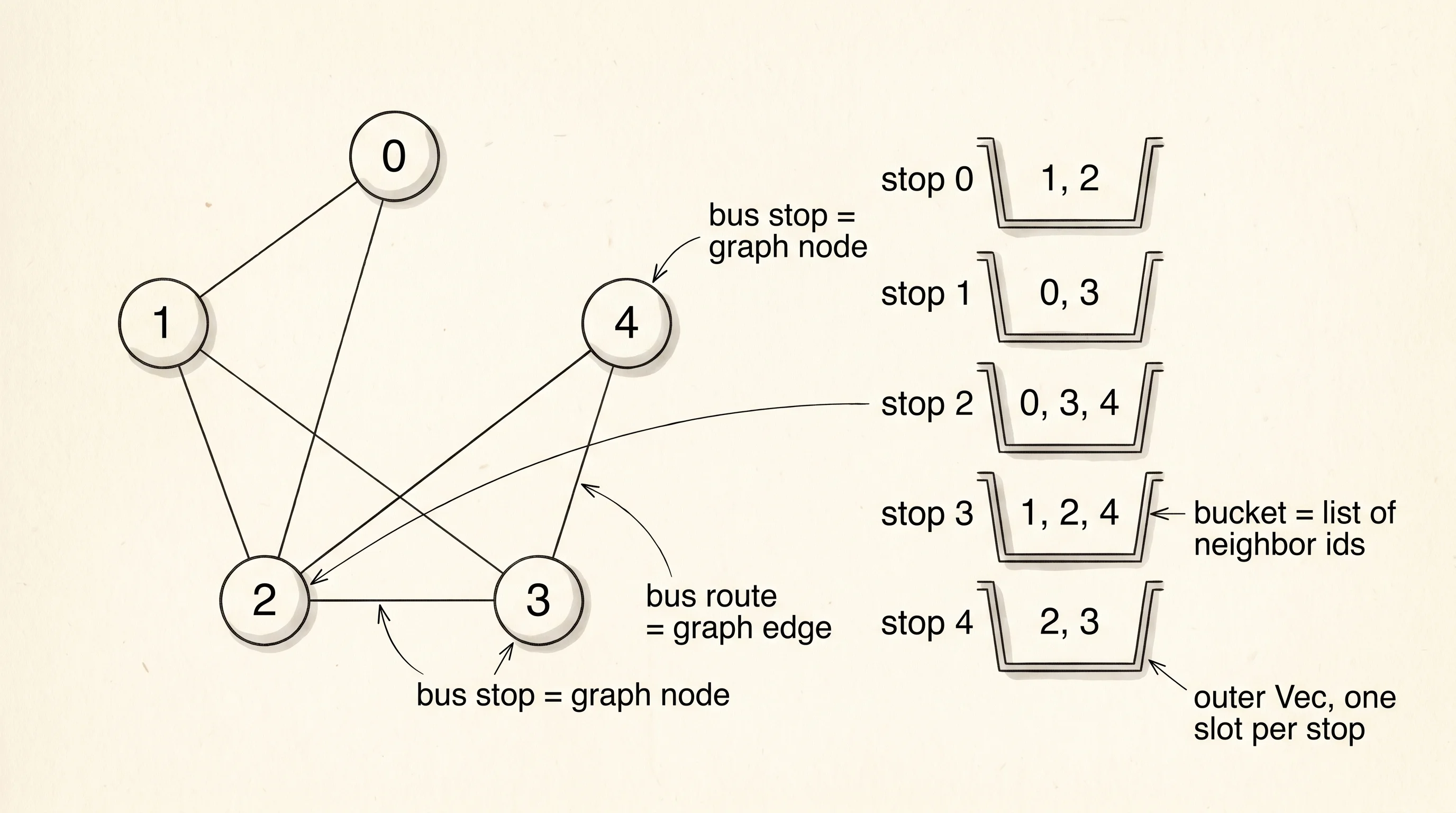
A graph in code is two things — a list of stops and, for each stop, a list of which other stops it connects to. The natural way to store that in Rust is Vec<Vec<usize>>. The outer Vec has one slot per stop. The inner Vec at position i lists every stop reachable in one ride from stop i. This shape is called an adjacency list. It is the bucket model. Each stop owns a bucket of neighbor numbers and nothing else.

fn build_town() -> Vec<Vec<usize>> {
    // 5 bus stops, 6 two-way routes.
    let edges: [(usize, usize); 6] = [(0, 1), (0, 2), (1, 3), (2, 3), (2, 4), (3, 4)];
    let stop_count = 5;
    let mut routes: Vec<Vec<usize>> = vec![Vec::new(); stop_count];
    for (a, b) in edges {
        routes[a].push(b);
        routes[b].push(a);
    }
    // Sort each bucket so the print order is the same on every machine.
    for bucket in routes.iter_mut() {
        bucket.sort();
    }
    routes
}

fn print_buckets(routes: &[Vec<usize>]) {
    println!("-- adjacency list (stop -> bucket of neighbors) --");
    for (stop, bucket) in routes.iter().enumerate() {
        println!("  stop {stop}: {bucket:?}");
    }
}

The town has 5 stops and 6 two-way routes. Routes go both directions, so when route (0, 1) exists, we push 1 into stop 0's bucket and 0 into stop 1's bucket. Sorting each bucket at the end is the kind of thing nobody bothers with in production code but matters here because a test snapshot has to print the same numbers in the same order on every machine. Otherwise the iteration order of the buckets would drift and the lesson would lie. The print_buckets function reads the outer Vec, enumerates it to pair each bucket with its stop number, and dumps the contents.

There is a second way to store a graph called an adjacency matrix. Instead of buckets, you build an n by n grid of zeros and ones. Cell (row, col) is 1 if a route exists between row and col, otherwise 0. The matrix is fast to ask "is there a direct route from stop 2 to stop 4?" — one lookup. It is wasteful when the graph is sparse, because most of the cells are zero. Most real-world graphs are sparse — the average person on Facebook has a few hundred friends, not three billion — so adjacency lists win in practice. The matrix is still useful to see, because looking at the grid makes the symmetry of an undirected graph obvious.

fn print_matrix(routes: &[Vec<usize>]) {
    let n = routes.len();
    println!("-- adjacency matrix ({n} by {n} grid) --");
    print!("     ");
    for col in 0..n {
        print!(" {col}");
    }
    println!();
    for row in 0..n {
        print!("  {row}: ");
        for col in 0..n {
            let connected = routes[row].contains(&col);
            print!(" {}", if connected { 1 } else { 0 });
        }
        println!();
    }
}

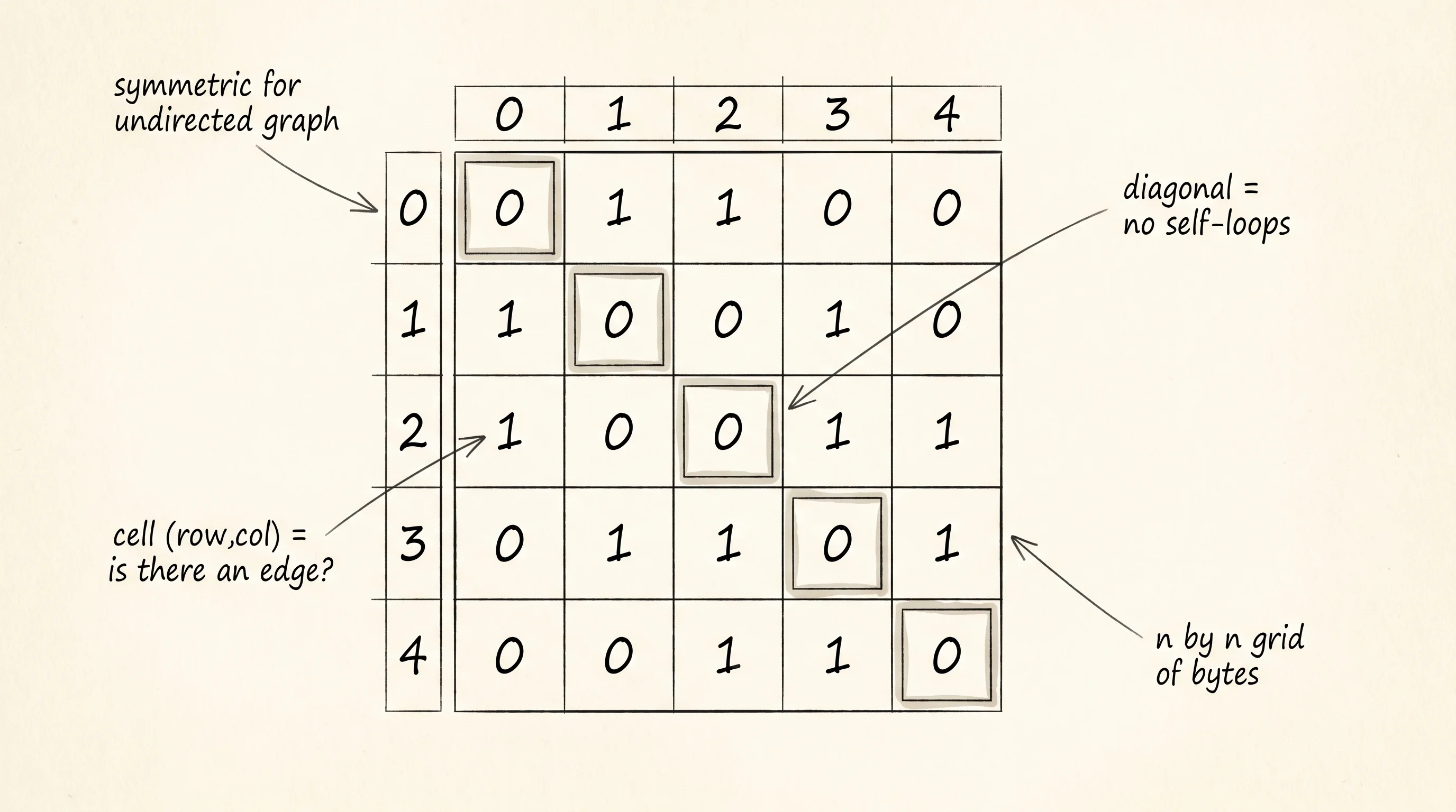
Read the printed matrix in the output below. The diagonal is all zeros because no stop has a route to itself. The grid is symmetric across the diagonal — if (2, 4) is a 1, then (4, 2) is a 1, because a two-way route works both ways. If the routes were one-way buses, the grid would not be symmetric.

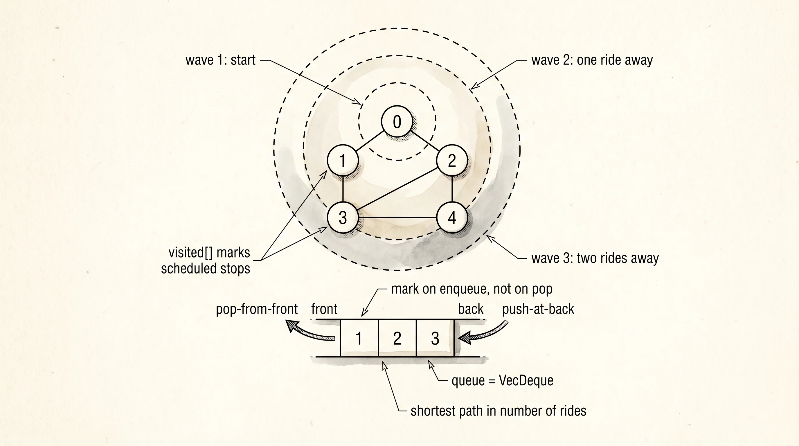
Once the graph is built, the question that comes up over and over is — starting from one stop, in what order do I visit the rest? The answer depends on how you walk. Breadth-first search is the dispatcher approach. You stand at stop 0 with a clipboard. You write down every neighbor of stop 0 and mark them as scheduled. Then you walk to the first scheduled stop, write down its unscheduled neighbors at the bottom of your list, and walk to the next scheduled stop. The clipboard is processed in order from top to bottom — first-in, first-out. The stops you visit move outward in waves. Wave 1 is stop 0. Wave 2 is everyone one ride away. Wave 3 is everyone two rides away. The data structure that holds the clipboard is a queue. Rust's standard library ships one called VecDeque — a ring buffer with cheap push-back and pop-front, exactly the shape you need.

fn bfs(routes: &[Vec<usize>], start: usize) -> Vec<usize> {
    let mut visited = vec![false; routes.len()];
    let mut queue: VecDeque<usize> = VecDeque::new();
    let mut order: Vec<usize> = Vec::new();

    visited[start] = true;
    queue.push_back(start);
    println!("  enqueue {start}  queue={:?}", queue);

    while let Some(stop) = queue.pop_front() {
        order.push(stop);
        println!("  visit   {stop}  queue={:?}", queue);
        for &next in &routes[stop] {
            if !visited[next] {
                visited[next] = true;
                queue.push_back(next);
                println!("  enqueue {next}  queue={:?}", queue);
            }
        }
    }
    order
}

The visited vector is a 5-slot array of bool so we never schedule the same stop twice. The queue starts with the start stop. The loop pops the front, prints it as visited, then walks the bucket of neighbors. For each neighbor that has not been visited, we mark it visited the moment we schedule it, not when we pop it. That detail matters. If you waited to mark a stop visited until you popped it, you would enqueue it three or four times before getting to it, and the queue would explode. Marking on enqueue is the rule. Every stop goes into the queue at most once.

Run the program.

-- adjacency list (stop -> bucket of neighbors) --
  stop 0: [1, 2]
  stop 1: [0, 3]
  stop 2: [0, 3, 4]
  stop 3: [1, 2, 4]
  stop 4: [2, 3]

-- adjacency matrix (5 by 5 grid) --
      0 1 2 3 4
  0:  0 1 1 0 0
  1:  1 0 0 1 0
  2:  1 0 0 1 1
  3:  0 1 1 0 1
  4:  0 0 1 1 0

-- BFS from stop 0 (visit order, wave by wave) --
  enqueue 0  queue=[0]
  visit   0  queue=[]
  enqueue 1  queue=[1]
  enqueue 2  queue=[1, 2]
  visit   1  queue=[2]
  enqueue 3  queue=[2, 3]
  visit   2  queue=[3]
  enqueue 4  queue=[3, 4]
  visit   3  queue=[4]
  visit   4  queue=[]
BFS visit order: [0, 1, 2, 3, 4]

-- DFS from stop 0 (follow one trail to the end first) --
DFS visit order: [0, 1, 3, 2, 4]

Look at the BFS trace in the middle of the output. The queue is printed after every push and every pop, so you can watch the wavefront. Stop 0 goes in alone. We pop 0 and enqueue its neighbors 1 and 2. We pop 1 and enqueue 3. We pop 2 and enqueue 4. We pop 3, whose neighbors 1, 2, and 4 are already visited, so nothing new gets scheduled. We pop 4. The final visit order is [0, 1, 2, 3, 4] — first the start, then everything one ride away, then everything two rides away. BFS gives you the shortest path in number of rides from the start to every other stop, for free, because of the wave shape.

There is a sibling algorithm called depth-first search that swaps the queue for a stack. Instead of fanning outward in waves, it follows one trail as deep as it goes, then backs up and tries the next. Same visited bookkeeping. Same neighbor lists. Different data structure — a Vec used as a stack with push and pop. Look at the DFS line at the bottom of the output: [0, 1, 3, 2, 4]. The walker started at 0, went to 1, then dove to 3, then to 2, then to 4. It never split into a wave. BFS is for shortest path. DFS is for "have I seen this whole connected piece?" and for things like topological sorts where you need to find the last reachable node first.

A question worth answering before moving on. Why did the DFS in the output visit 3 before 2, even though 2 has a smaller number? Because DFS pops the most recently pushed item. The code pushes neighbors in reverse order so the smallest id ends up on top of the stack. Stop 0's neighbors are [1, 2] — pushed in reverse, that is 2 then 1, leaving 1 on top. We pop 1. Stop 1's neighbors are [0, 3] — 0 is visited, 3 gets pushed. We pop 3. From 3 we push its unvisited neighbors. The walker is in a tunnel, not on a wave.

Everything above is Vec<Vec<usize>> and a queue. It is enough for a friendship graph or a small town. The moment graphs get serious — millions of nodes, weighted edges, finding the shortest weighted path with Dijkstra, finding cycles, finding minimum spanning trees — people reach for a crate called petgraph. It is the Rust ecosystem's default graph library. Inside petgraph you get a real Graph<N, E> type where nodes carry data of type N and edges carry data of type E, plus battle-tested implementations of Dijkstra, A-star, Bellman-Ford, Kosaraju's strongly connected components, and a way to dump the graph to Graphviz dot format for rendering. The point of building the graph by hand first is that when you open petgraph later, you will read the source and recognize every move — the adjacency list is still there, the BFS is still using a queue, the only difference is generics and polish. Lessons in the algorithms section will reach for petgraph once we have built enough by hand to read its source without flinching.

A graph in a Vec<Vec<usize>> has one weakness — every edge is a number, with no payload. You cannot ask "how long is the ride from stop 2 to stop 4?" because the edges have no weights. The next lesson teaches weighted graphs and Dijkstra's shortest-path algorithm, which is the moment the queue grows up into a priority queue.