B-trees

A B-tree is a phonebook with thick index tabs. Open the binder and the first sheet you see is not a single name — it is a whole row of dividers reading "A–F", "G–M", "N–S", "T–Z". You scan the row, pick the one tab that covers your name, flip to it, and the page behind that tab is itself another row of finer dividers. After two or three flips you are on the leaf page that holds the actual entry. The binder works because each index sheet holds many dividers at once, so even a phonebook with millions of names only needs a handful of flips to land on any single name. The trick is the fat sheet, not the tall tower.

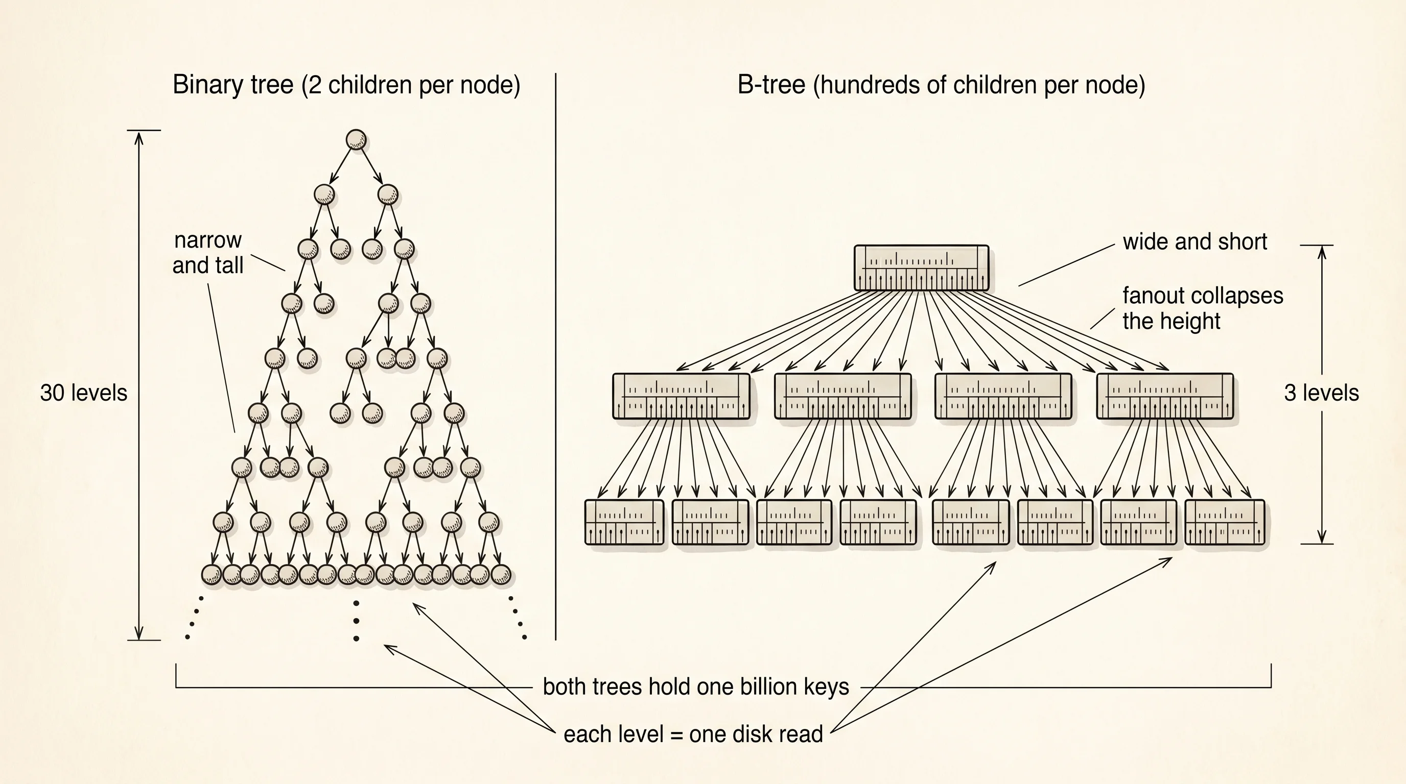
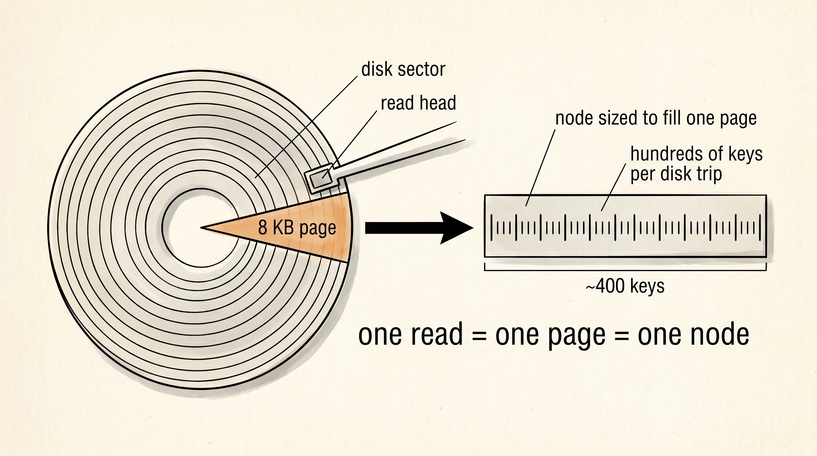
The reason this shape exists is a bottleneck Rudolf Bayer and Edward McCreight hit at Boeing in 1971. They were storing records on spinning disks, and a disk does not hand you a single byte — it hands you a whole page of about 4 kilobytes, because the read head has to swing to the right track and wait for the right spot to come around under it. That swing is roughly a million times slower than a single arithmetic step. A normal binary tree puts one key per node and two children, so a tree of a billion keys is 30 nodes tall, which means 30 disk swings to find anything. Bayer and McCreight asked the obvious question. If we pay for a whole page every time we touch the disk, why not stuff hundreds of keys into each page and let one node have hundreds of children instead of two? The tree gets fat in the middle and short top-to-bottom. A B-tree of a billion keys is three or four pages tall. Three swings instead of thirty. Their paper is the reason every serious database — PostgreSQL, SQLite, MySQL, Oracle — stores its indexes as B-trees on disk to this day.

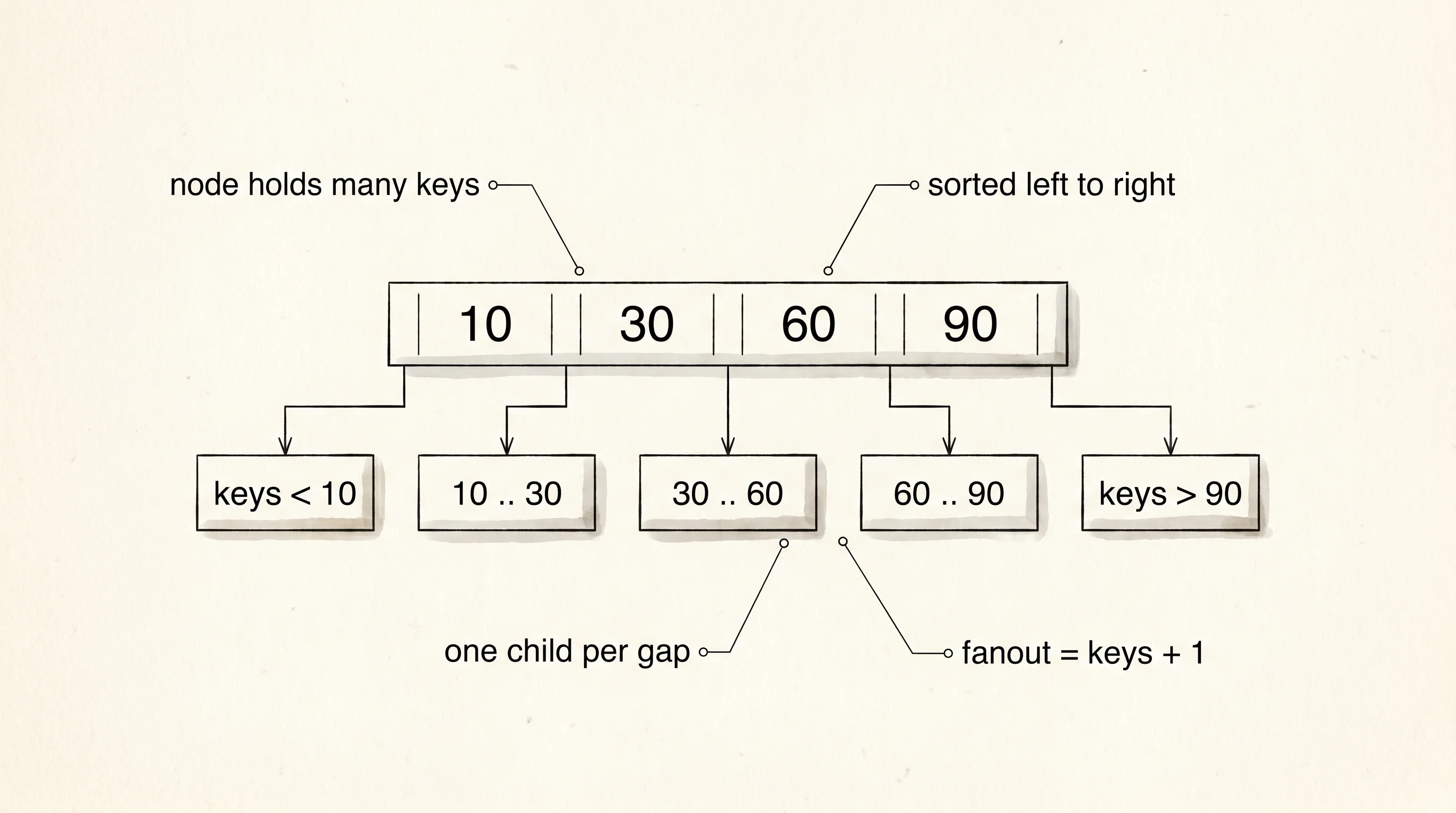
The shape of one B-tree node is easy to sketch in Rust even though writing a full implementation is a graduate project. A node holds a sorted vector of keys and a vector of child links sitting between those keys. If the keys are 10, 30, and 60, the four children cover everything below 10, everything between 10 and 30, everything between 30 and 60, and everything above 60. You walk down by comparing your target against the keys on the current page and following the matching gap. Here is the type the way the reader should picture it — no working code, just the shape.

// Illustrative shape of one B-tree node. The real std::collections::BTreeMap
// uses a tuned, unsafe layout for cache performance — this struct is only
// here so the reader can picture a node holding many keys at once.
#[allow(dead_code)]
struct BTreeNode {
    keys: Vec<i32>,
    children: Vec<Box<BTreeNode>>,
}

The reader does not have to build one from scratch. The Rust standard library ships std::collections::BTreeMap, which is a B-tree tuned for memory instead of disk — the nodes are sized to fit a few cache lines rather than a disk page, but the idea is the same. Each internal node holds many keys, the tree stays short, and lookups follow the divider tabs. Insert keys in whatever order you want and the map keeps them sorted automatically. That last bit is the part HashMap cannot do. A hash table scatters keys to random buckets — fast for "is this key in here?" but useless for "give me everything between 10 and 50." A BTreeMap keeps the spine of the phonebook in order, so a range query is just a finger walking across pages.

fn build_phonebook() -> BTreeMap<i32, &'static str> {
    let mut phonebook: BTreeMap<i32, &'static str> = BTreeMap::new();
    let entries = [
        (42, "diana"),
        (7, "alice"),
        (15, "bob"),
        (99, "frank"),
        (3, "amir"),
        (61, "elena"),
        (28, "carlos"),
        (50, "dmitri"),
    ];
    for (page, name) in entries {
        phonebook.insert(page, name);
    }
    phonebook
}

fn show_in_order(phonebook: &BTreeMap<i32, &'static str>) {
    for (page, name) in phonebook {
        println!("page {page:>3}: {name}");
    }
}

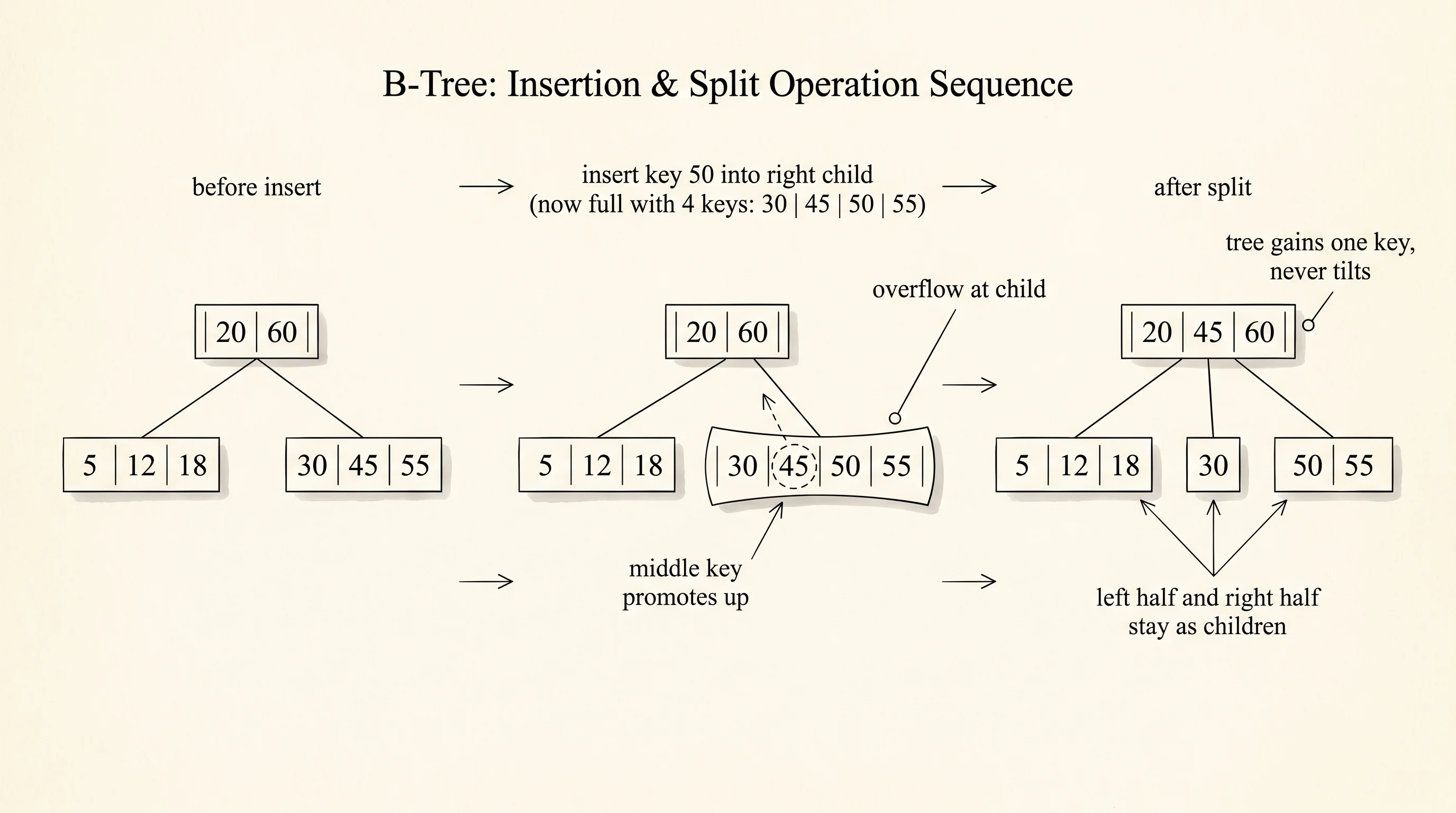
We insert eight name entries with random-looking page numbers — 42, 7, 15, 99, 3, 61, 28, 50. The insert calls do not preserve insertion order. The map sorts the keys behind the scenes by finding the right node, slotting the key into the right position in that node's key vector, and splitting the node into two if it overflows. That split is the rule that keeps the tree balanced. A node has a maximum number of keys, say 4 in a teaching example or hundreds in a real database. When you cram in one too many, the node breaks down the middle. The middle key goes up to the parent as a new divider. The left half stays as one child, the right half becomes another. The tree gains a key in the parent and a node, never gets crooked, and never gets taller except when the root itself splits — which is the only operation that adds a level.

Walking the map prints the entries in sorted order. The reader sees that order in the first block of output.

-- inserted out of order, walked in order --
page   3: amir
page   7: alice
page  15: bob
page  28: carlos
page  42: diana
page  50: dmitri
page  61: elena
page  99: frank

-- range queries are a sliced walk, not a re-sort --
pages 10..50:
  page  15: bob
  page  28: carlos
  page  42: diana

pages 60..100:
  page  61: elena
  page  99: frank

Look at the first block. The numbers come out 3, 7, 15, 28, 42, 50, 61, 99 — strictly ascending — even though we inserted them in the order 42, 7, 15, 99, 3, 61, 28, 50. The map paid the sort cost on each insert, not at print time. The second part of the program shows what the order is good for. phonebook.range(10..50) walks straight to the first key at or above 10 and stops at 50, handing back exactly the entries in between. There is no scan of the whole map. The tree knows where the range starts because finding key 10 takes the same flip-flip-flip walk down the dividers as finding any other key. Once the cursor is parked on page 15, it just steps forward in sorted order until it sees 50.

A question worth asking. Why does the range output skip page 50 even though the entry exists? Because Rust's range syntax 10..50 is half-open — lower bound included, upper bound excluded. That convention falls out of .. meaning "up to but not including." If you want both ends inclusive, you write 10..=50 and the map will include the entry at 50. The B-tree does not care which kind of range you hand it; it just walks until the cursor passes the upper bound.

fn show_range(phonebook: &BTreeMap<i32, &'static str>, lo: i32, hi: i32) {
    println!("pages {lo}..{hi}:");
    for (page, name) in phonebook.range(lo..hi) {
        println!("  page {page:>3}: {name}");
    }
}

The phonebook analogy carries one more piece of weight. When std::collections::BTreeMap is in memory, each node is sized to fit comfortably in a CPU cache line — maybe 6 to 11 keys per node depending on the value size. When PostgreSQL's index is sitting on a spinning disk or an SSD, each node is sized to fit exactly one disk page, around 8 kilobytes, which is hundreds of keys per node. The structure is the same. The number that changes is how fat each page of the binder is. A bigger page means more dividers per sheet, which means fewer sheets to flip through, which means fewer slow trips to the disk. Bayer and McCreight saw the trade-off in 1971 and the curve has held ever since — every time storage gets a new kind of hardware, the only thing that changes about B-trees is the page size that makes the math work out.

The B-tree is the right shape when keys are comparable and the queries are point lookups or ranges. It is the wrong shape when keys are not comparable — a user ID hash, a content fingerprint, a UUID with no meaningful order — and the only queries are "do you have this exact key." The next lesson takes the keys out of order on purpose and asks how a structure can find any of them in constant time without ever comparing one key to another.