Big O, in Microseconds

The title of this lesson is a half-truth. Big O is not about microseconds. Big O is about a page flip. Imagine a phone book with 4096 pages, names in order from A to Z, and you need to find one person. You could open page 1, read it, flip to page 2, read it, flip to page 3, and grind through the whole book. Or you could open the book to the middle, glance at the page, decide whether your person is in the front half or the back half, and throw away the half you do not need. Big O is just a way to count page flips. It does not care how fast your fingers are or how warm your room is. It cares how many flips you do as the book gets thicker.

The wall-clock numbers a microsecond timer would give you depend on the laptop you ran the code on, what else was running, whether the CPU was hot. None of that helps anyone reading the lesson on a different machine a year from now. So this lesson cheats — it counts the operations the algorithm does, not the time the operations take. An operation is one page flip. Pass a &mut u64 counter into each function, bump it every time the algorithm compares two items, and the count comes out byte-identical no matter who runs the code. That is the stand-in. The shape of how the count grows as the book gets thicker is the thing Big O names.

The notation itself is older than computers by 64 years. A German number theorist named Paul Bachmann wrote down the big-O symbol in 1894 to talk about how fast prime-counting functions grew. Edmund Landau picked it up in 1909 and the symbol became a standard tool in pure math. None of it had anything to do with code. Then in 1976 Donald Knuth, halfway through writing The Art of Computer Programming at Stanford, looked at how his colleagues described algorithm cost — half of them said "fast," the other half said "slow," nobody could agree — and he reached over to the math department and grabbed the big-O symbol that was already lying there. He published a one-page note saying we should use it, and within two years every algorithms textbook was written in Big O. The trick was not invention. The trick was naming.

The two algorithms that show the gap most clearly are the two ways to find a name in the phone book. Linear search opens to page 1 and flips one at a time. Binary search opens to the middle and halves the search range each time.

fn linear_search(haystack: &[u32], needle: u32, ops: &mut u64) -> Option<usize> {
    for (i, item) in haystack.iter().enumerate() {
        *ops += 1;
        if *item == needle {
            return Some(i);
        }
    }
    None
}

fn binary_search(haystack: &[u32], needle: u32, ops: &mut u64) -> Option<usize> {
    let mut lo = 0usize;
    let mut hi = haystack.len();
    while lo < hi {
        *ops += 1;
        let mid = lo + (hi - lo) / 2;
        if haystack[mid] == needle {
            return Some(mid);
        } else if haystack[mid] < needle {
            lo = mid + 1;
        } else {
            hi = mid;
        }
    }
    None
}

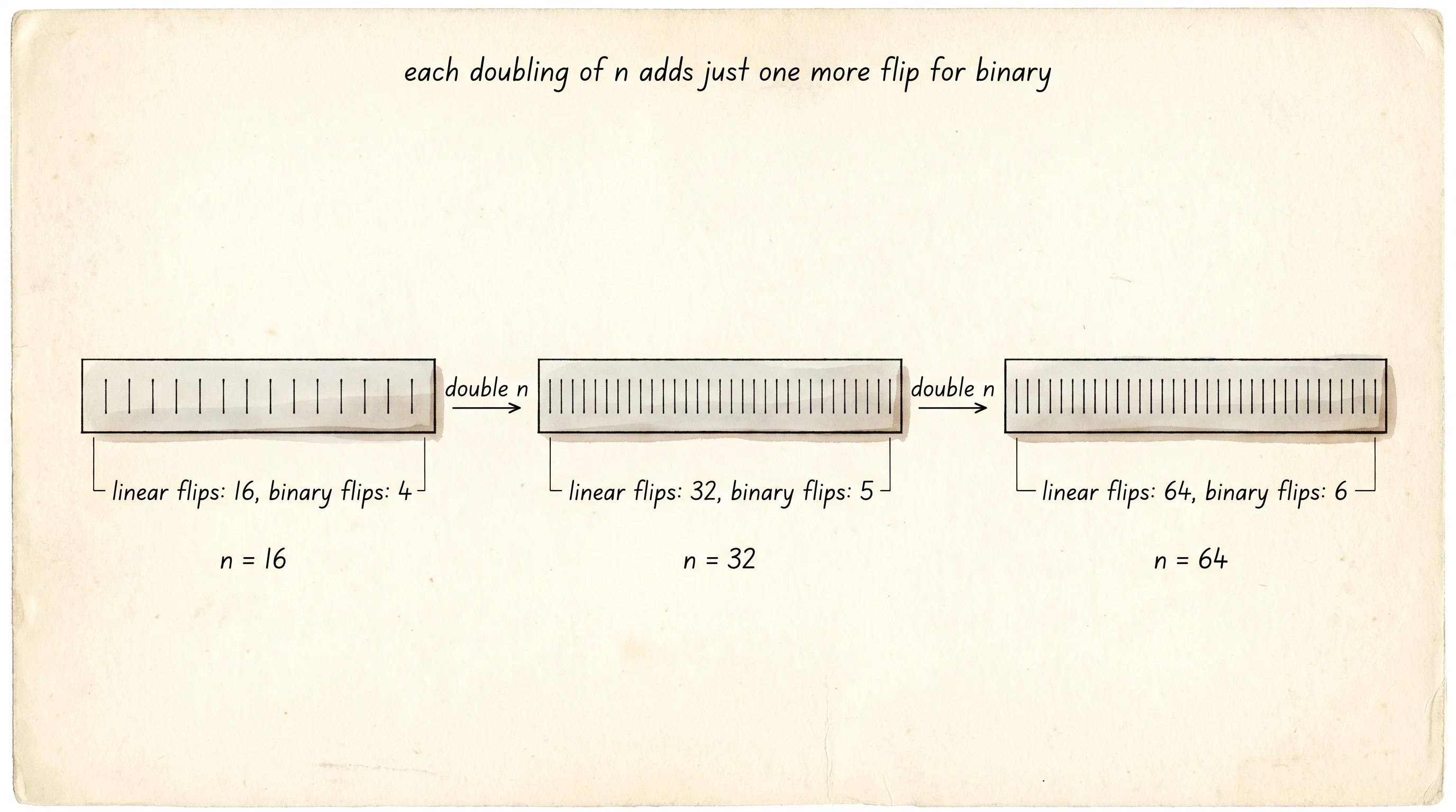
Read both functions side by side. linear_search walks the slice from index 0, bumps the counter once per item it inspects, and returns the index when it finds the needle. binary_search keeps a lo and hi window, picks the middle, bumps the counter once per check, and shrinks the window by half each iteration. The body of linear_search runs once per item. The body of binary_search runs once per halving. If you double the size of the book, linear search has to flip twice as many pages. Binary search adds one more halving — one more flip.

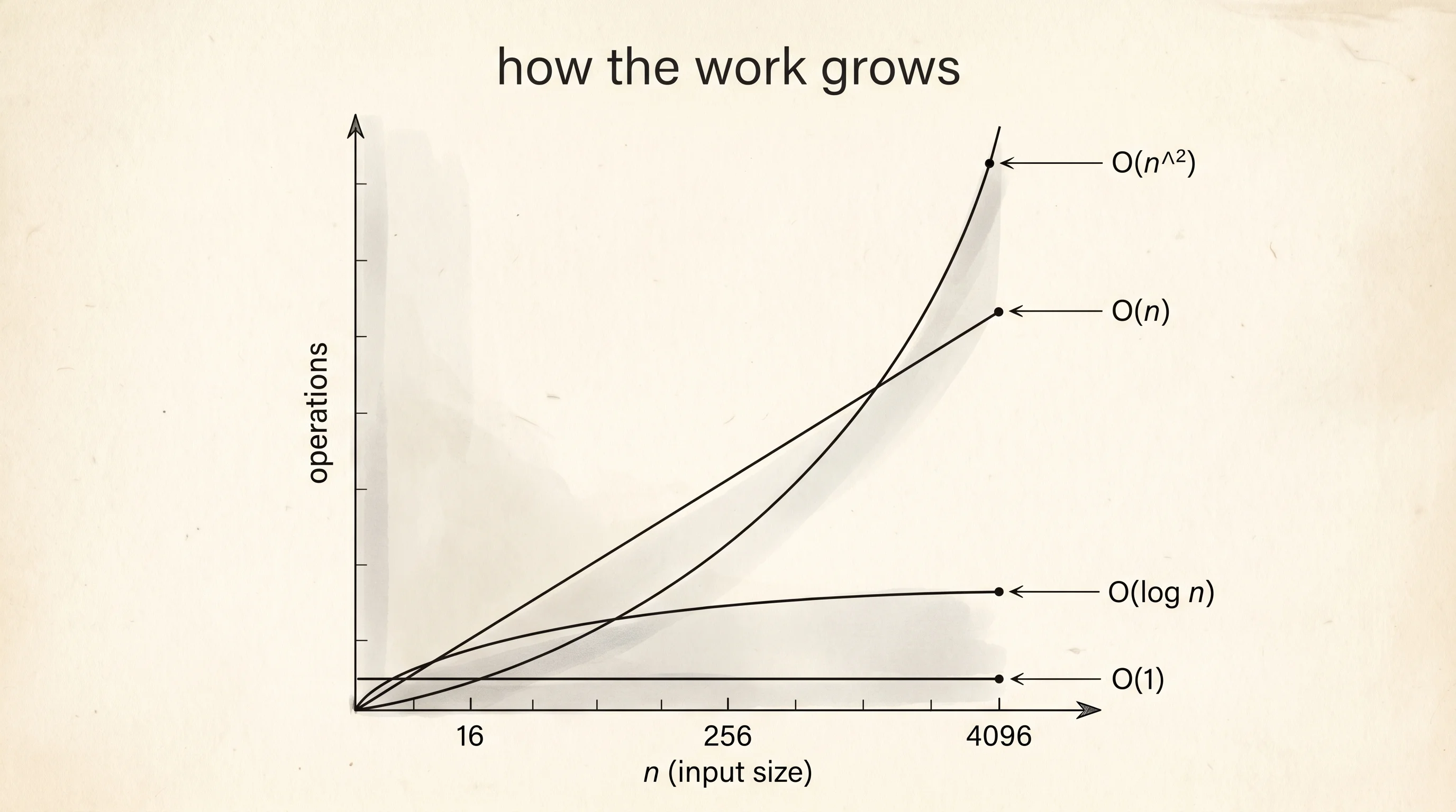
That is the whole difference. Linear is O(n) because the count grows in step with n. Binary is O(log n) because each step throws away half the remaining pages, so the count grows like the number of times you can cut n in half before nothing is left. For n=4096, log₂(4096) is 12. For a book a million pages long, log₂(1,000,000) is 20. For a book the size of the internet, it is around 40. Linear would have flipped a million pages to find what binary finds in 20.

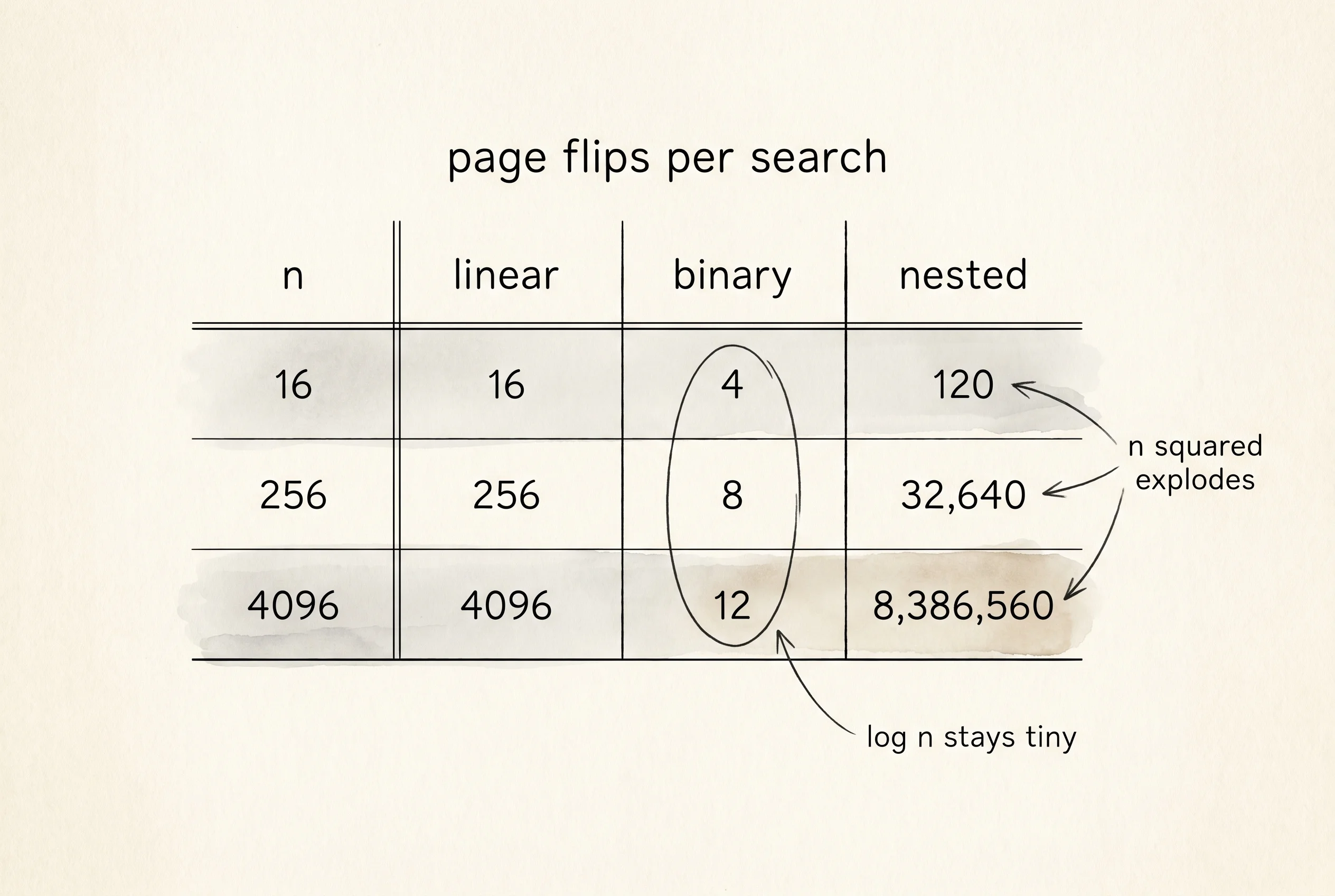
The slower shapes get worse fast. O(n²) is what happens when you look at every pair of items in a list — the nested loop where every page is compared to every other page. For n=16 that is 120 comparisons. For n=256 it is 32,640. For n=4096 it is 8.3 million. O(n log n) is what happens when you sort the book first and then walk it once — sorting itself takes about n times log n comparisons, then the walk adds n more. For n=4096 that is around 53,000 — much less than the 8.3 million of O(n²), but still much more than the 12 of binary search.

fn nested_pair_count(items: &[u32], ops: &mut u64) -> u64 {
    let mut pairs = 0u64;
    for i in 0..items.len() {
        for j in (i + 1)..items.len() {
            *ops += 1;
            if items[i] + items[j] == 100 {
                pairs += 1;
            }
        }
    }
    pairs
}

fn sort_then_walk(items: &mut [u32], ops: &mut u64) -> u32 {
    let n = items.len();
    if n == 0 {
        return 0;
    }
    items.sort();
    // sort cost: count n * log2(n) comparisons as a stand-in.
    let log2 = (usize::BITS - n.next_power_of_two().leading_zeros() - 1) as u64;
    *ops += (n as u64) * log2.max(1);
    let mut largest = items[0];
    for v in items.iter() {
        *ops += 1;
        if *v > largest {
            largest = *v;
        }
    }
    largest
}

The nested_pair_count function is two for-loops, one inside the other. The outer one walks indices 0 through n-1, the inner one walks indices i+1 through n-1, and the counter bumps once per inner step. The total count is n times n-1 divided by 2, which is about n² for large n. The sort_then_walk function uses the standard library sort, then estimates the sort cost as n times log₂(n) — that is the well-known shape of an optimal comparison sort — and adds one bump per item during the walk. Those four functions cover the four shapes that show up in 90 percent of code you will ever read.

The driver runs each algorithm on the same input at sizes 16, 256, and 4096, and prints a single row per size.

fn make_sorted_input(n: usize) -> Vec<u32> {
    (0..n as u32).collect()
}

fn run_size(n: usize) {
    let data = make_sorted_input(n);
    let needle = (n as u32) - 1;

    let mut linear_ops = 0u64;
    linear_search(&data, needle, &mut linear_ops);

    let mut binary_ops = 0u64;
    binary_search(&data, needle, &mut binary_ops);

    let mut nested_ops = 0u64;
    nested_pair_count(&data, &mut nested_ops);

    let mut walk_ops = 0u64;
    let mut copy = data.clone();
    sort_then_walk(&mut copy, &mut walk_ops);

    println!(
        "n={n:>5}  linear={linear_ops:>10}  binary={binary_ops:>4}  nested={nested_ops:>10}  sort+walk={walk_ops:>10}"
    );
}

The needle is set to the last element of the sorted input — the worst case for linear search, because it has to flip every page before finding the needle. Binary search does not care about which element you ask for. Its count depends only on the size of the book, not on what is inside. That property is why binary search is the workhorse of every database index ever built. Stick the data in sorted order and finding any one item takes log n flips, no matter who is asking or what they are looking for.

fn main() {
    println!("counting operations for each algorithm shape:");
    println!("(linear=O(n), binary=O(log n), nested=O(n^2), sort+walk=O(n log n))");
    println!();
    for n in [16usize, 256, 4096] {
        run_size(n);
    }
}

Run the program and read the table top to bottom.

counting operations for each algorithm shape:
(linear=O(n), binary=O(log n), nested=O(n^2), sort+walk=O(n log n))

n=   16  linear=        16  binary=   4  nested=       120  sort+walk=        80
n=  256  linear=       256  binary=   8  nested=     32640  sort+walk=      2304
n= 4096  linear=      4096  binary=  12  nested=   8386560  sort+walk=     53248

The linear column doubles when n doubles. Look at the first to the second row — 16 to 256 is a 16× increase, and 16 to 256 is exactly the same 16× jump in linear ops. The binary column adds four when n goes from 16 to 256, because 256 is 16 doubled four times. From 256 to 4096 it adds another four. That is what log n looks like — a slow drip, never more than a handful even when n explodes. The nested column is the horror story. 120 to 32,640 to 8.3 million. Every time you make the book 16× thicker, the work goes up 256× — that is n squared in plain sight. The sort+walk column splits the difference. It is bad, but it is not nested-loop bad. It is good enough that every general-purpose sort in every language uses an algorithm of this shape.

One question to sit with. The binary search row went 4, 8, 12 across sizes 16, 256, 4096. Why are those numbers exactly four apart? Because each step of the size — 16 to 256, 256 to 4096 — multiplies n by 16, which is 2 to the fourth, which means you can cut the new range in half four more times before it is empty. That is the whole secret of logarithms in one sentence. Each multiplication of the input is an addition for log.

What Big O cannot tell you is the constant factor — whether one O(n) algorithm runs ten times faster than another O(n) algorithm on the same hardware because of cache behavior, branch prediction, or how friendly the loop is to the CPU. Counting page flips ignores all of that. The next lesson digs into one specific shape, sorting, and asks why four different O(n log n) algorithms can have wildly different real-world speeds even though Big O calls them all the same.