Time-Series Basics

A bakery owner walks in at the end of every hour and writes a number on a clipboard — how many people came through the door. By the end of the day she has 24 numbers in a column. The numbers wiggle. They are low at dawn, climb toward lunch, peak in the afternoon, slide back down by evening. The real question is never any single number. The real question is the shape of the day and what tomorrow's shape will look like, because the answer decides how much dough she mixes at 5 a.m.

That clipboard is a time series — values lined up against the clock, where the order matters. Order matters because the value at 2 p.m. is connected to the value at 1 p.m. in a way that the price of milk in Ohio is not. The earliest people who took this seriously were actuaries and astronomers in the 1800s tracking sunspots and life-expectancy tables, and the first big break came in 1927 when the Yule family ran into a problem fitting curves to those sunspot counts. He realized you could predict the next value from a weighted blend of the previous values, and the field of time-series analysis was born. By the 1960s a pair of statisticians named Box and Jenkins had packaged the idea into a recipe called ARIMA, and a few years later Holt and Winters added pieces that handled seasonal swings. None of this is what the bakery owner needs at the counter. She needs three short tricks that any clipboard reader can run by hand, and those three tricks are what this lesson covers.

Start by laying the 24 numbers on the table.

const HOURS: [&str; 24] = [
    "00", "01", "02", "03", "04", "05", "06", "07", "08", "09", "10", "11", "12", "13", "14", "15",
    "16", "17", "18", "19", "20", "21", "22", "23",
];

const TEMP_F: [f64; 24] = [
    52.0, 51.0, 50.0, 49.0, 49.0, 50.0, 53.0, 57.0, 62.0, 66.0, 70.0, 73.0, 75.0, 76.0, 76.0, 75.0,
    73.0, 70.0, 66.0, 62.0, 59.0, 57.0, 55.0, 53.0,
];

The HOURS array is a stripe of labels and the TEMP_F array is the series itself — 24 daytime temperatures in Fahrenheit standing in for any hourly count. Holding the values in &[f64] is the cheapest container the math can ride on, and pairing them with the labels through zip later keeps the printout honest. Print the raw column first so the eye can see the shape before the math touches it.

fn show_series() {
    println!("--- raw series ---");
    for (h, t) in HOURS.iter().zip(TEMP_F.iter()) {
        println!("{}h  {:.4}", h, t);
    }
    println!();
}

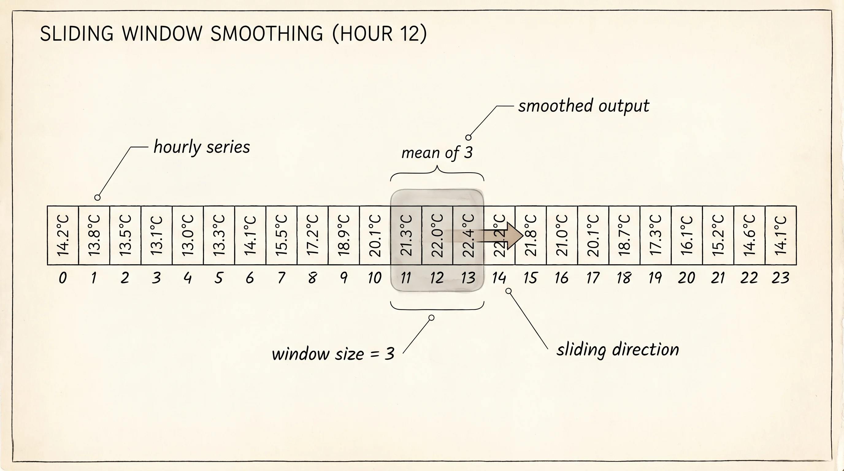
The owner stares at the raw column and sees a problem. The dip at hour 4 was probably a delivery truck blocking the door. The bump at hour 13 was probably a tour bus. Both are noise on top of the real shape. The first tool fixes this — a rolling mean.

fn rolling_mean(series: &[f64], window: usize) -> Vec<Option<f64>> {
    let mut out = Vec::with_capacity(series.len());
    for i in 0..series.len() {
        if i + 1 < window {
            out.push(None);
        } else {
            let slice = &series[i + 1 - window..=i];
            let sum: f64 = slice.iter().sum();
            out.push(Some(sum / window as f64));
        }
    }
    out
}

fn show_rolling_mean() {
    let smoothed = rolling_mean(&TEMP_F, 3);
    println!("--- rolling mean (window=3) ---");
    for (h, v) in HOURS.iter().zip(smoothed.iter()) {
        match v {
            Some(x) => println!("{}h  {:.4}", h, x),
            None => println!("{}h  (warmup)", h),
        }
    }
    println!();
}

A rolling mean with a window of 3 says — at every hour, take this hour and the 2 before it, add them up, divide by 3. That is the value for this hour in the smoothed series. The first 2 hours have no answer because there are not yet 3 values to average, which the code marks with None so the reader can see the warmup window honestly instead of inventing a number. The window slides forward one step at a time and the average glides with it. Delivery trucks get diluted. Tour buses get diluted. The underlying climb-and-fall of the day rises out of the fog.

The second tool answers a different question — not "what is the smoothed level" but "how much did we move this hour."

fn lag_one_diffs(series: &[f64]) -> Vec<Option<f64>> {
    let mut out = Vec::with_capacity(series.len());
    out.push(None);
    for i in 1..series.len() {
        out.push(Some(series[i] - series[i - 1]));
    }
    out
}

fn show_lag_diffs() {
    let diffs = lag_one_diffs(&TEMP_F);
    println!("--- lag-1 differences ---");
    for (h, d) in HOURS.iter().zip(diffs.iter()) {
        match d {
            Some(x) => println!("{}h  {:.4}", h, x),
            None => println!("{}h  (no prior)", h),
        }
    }
    println!();
}

A lag-1 difference is the simplest report a time series can give about itself. At hour i, subtract the value at hour i-1, and the answer is how far the count moved in that step. The first hour has no answer because there is no prior hour, so it sits as None. Positive numbers say the count is rising. Negative numbers say it is falling. A flat run of zeros says the day has plateaued. This single column is the bedrock under every fancier forecaster including ARIMA, where the "I" stands for "integrated" and means exactly this — work with the differences instead of the raw values, because differences are usually better behaved.

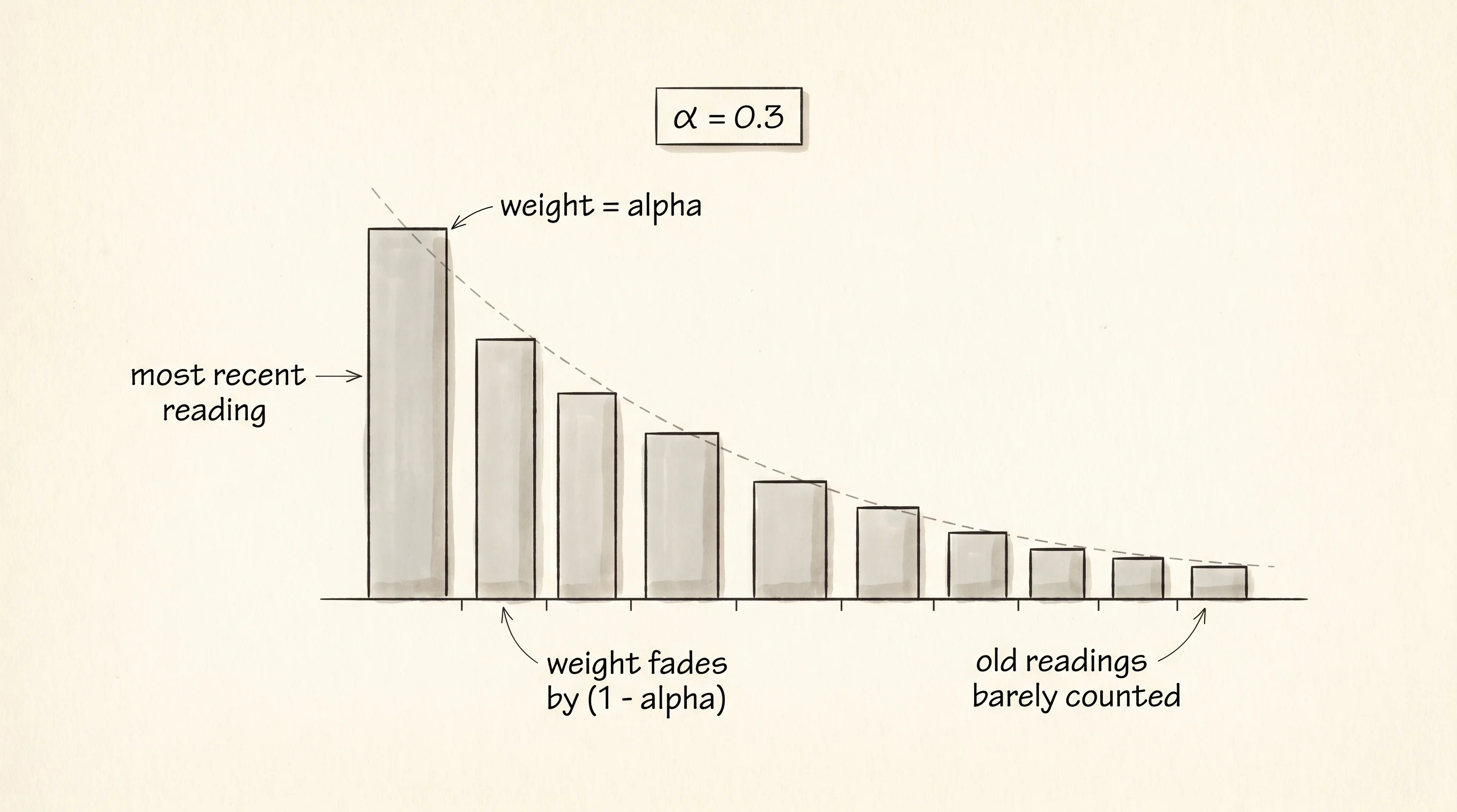
The third tool is the exponentially weighted moving average, or EWMA. The rolling mean treats every hour inside the window equally — the value 2 hours ago counts the same as the value right now. EWMA disagrees. It says the freshest value matters most, the one before it matters a little less, the one before that even less, and so on, with the importance fading as a clean geometric decay. A single number called alpha controls how fast the past fades. A high alpha listens hard to today. A low alpha trusts the long memory and barely reacts to a single odd hour.

fn ewma(series: &[f64], alpha: f64) -> Vec<f64> {
    let mut out = Vec::with_capacity(series.len());
    let mut level = series[0];
    out.push(level);
    for &x in &series[1..] {
        level = alpha * x + (1.0 - alpha) * level;
        out.push(level);
    }
    out
}

fn show_ewma() {
    let smoothed = ewma(&TEMP_F, 0.3);
    println!("--- ewma (alpha=0.3) ---");
    for (h, s) in HOURS.iter().zip(smoothed.iter()) {
        println!("{}h  {:.4}", h, s);
    }
    println!();
}

The formula is one line of arithmetic — level = alpha * x + (1 - alpha) * level. The new smoothed value is a blend of the new reading and the old smoothed value. With alpha = 0.3 the freshest hour gets 30 percent of the weight and the entire past gets the other 70 percent, with the importance of older readings falling off geometrically. This is the workhorse smoother that Holt published in 1957 while he was building inventory tools for the Office of Naval Research, and the same line of code shows up today inside trading systems, anomaly detectors, and the throttling logic of cell-tower controllers.

The last move is the one the owner cares about. What will the count be at hour 24, the hour that has not happened yet?

fn show_forecasts() {
    let last = *TEMP_F.last().expect("series is not empty");
    let smoothed = ewma(&TEMP_F, 0.3);
    let ses = *smoothed.last().expect("smoothed is not empty");
    println!("--- 1-step forecasts for hour 24 ---");
    println!("naive (carry last): {:.4}", last);
    println!("ses   (alpha=0.3) : {:.4}", ses);
}

The naive forecast carries the last value forward — whatever happened in the last hour will happen in the next hour. The simple exponential smoothing forecast hands back the most recent smoothed level — whatever the EWMA settled to, that is the prediction. Both forecasts are 1-step — they only commit to the very next hour, not the one after that. Naive is the floor every other forecaster has to beat. SES is the first floor a serious forecaster builds on top of naive, and it beats naive whenever the recent past has any signal beyond the single most recent point.

--- raw series ---
00h  52.0000
01h  51.0000
02h  50.0000
03h  49.0000
04h  49.0000
05h  50.0000
06h  53.0000
07h  57.0000
08h  62.0000
09h  66.0000
10h  70.0000
11h  73.0000
12h  75.0000
13h  76.0000
14h  76.0000
15h  75.0000
16h  73.0000
17h  70.0000
18h  66.0000
19h  62.0000
20h  59.0000
21h  57.0000
22h  55.0000
23h  53.0000

--- rolling mean (window=3) ---
00h  (warmup)
01h  (warmup)
02h  51.0000
03h  50.0000
04h  49.3333
05h  49.3333
06h  50.6667
07h  53.3333
08h  57.3333
09h  61.6667
10h  66.0000
11h  69.6667
12h  72.6667
13h  74.6667
14h  75.6667
15h  75.6667
16h  74.6667
17h  72.6667
18h  69.6667
19h  66.0000
20h  62.3333
21h  59.3333
22h  57.0000
23h  55.0000

--- lag-1 differences ---
00h  (no prior)
01h  -1.0000
02h  -1.0000
03h  -1.0000
04h  0.0000
05h  1.0000
06h  3.0000
07h  4.0000
08h  5.0000
09h  4.0000
10h  4.0000
11h  3.0000
12h  2.0000
13h  1.0000
14h  0.0000
15h  -1.0000
16h  -2.0000
17h  -3.0000
18h  -4.0000
19h  -4.0000
20h  -3.0000
21h  -2.0000
22h  -2.0000
23h  -2.0000

--- ewma (alpha=0.3) ---
00h  52.0000
01h  51.7000
02h  51.1900
03h  50.5330
04h  50.0731
05h  50.0512
06h  50.9358
07h  52.7551
08h  55.5286
09h  58.6700
10h  62.0690
11h  65.3483
12h  68.2438
13h  70.5707
14h  72.1995
15h  73.0396
16h  73.0277
17h  72.1194
18h  70.2836
19h  67.7985
20h  65.1590
21h  62.7113
22h  60.3979
23h  58.1785

--- 1-step forecasts for hour 24 ---
naive (carry last): 53.0000
ses   (alpha=0.3) : 58.1785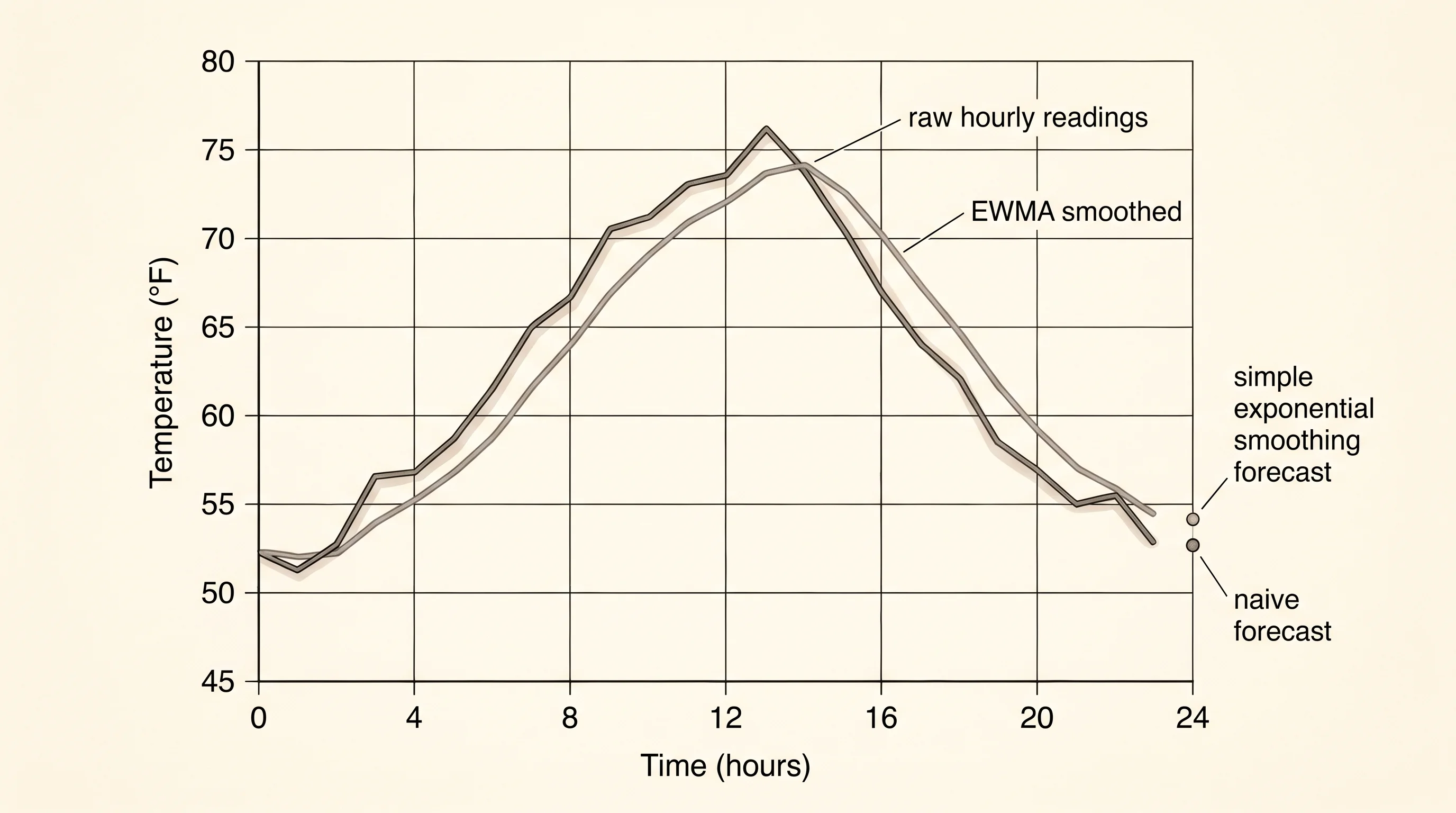

Read the output from the top. The raw column rises from 52 at midnight, peaks at 76 around 2 p.m., and slides back to 53 by 11 p.m. The rolling mean smooths the wiggle but lags the peak — its top sits between hours 12 and 14 instead of right on 13, which is what averaging the past always does. The lag-1 differences show the day in motion — positive numbers through the morning, zeros at the peak, negative numbers through the evening. The EWMA traces a curve close to the rolling mean but reacts a little faster on the way up and a little slower on the way down because the most recent values pull on it the hardest. At the bottom, the two forecasts disagree by 5 degrees — naive says 53, SES says 58.1785 — because SES still remembers the warm afternoon and naive does not.

One question worth asking — why does naive ever win, given how dumb it sounds? The reason is that on a series with no signal at all, like the daily price change of a stock, the next value really is best guessed as the current value, and any cleverer model adds noise instead of removing it. The forecaster who wins the most contests is the one who knows when to use naive and when to upgrade.

The thing this lesson cannot do is handle the seasonal swing that returns every 24 hours, every 7 days, or every 365 days, where the bakery is busy every Saturday at noon regardless of what last Tuesday looked like — which is the bottleneck Holt-Winters and the full ARIMA family solve.