Statistics You Actually Need

A coffee cart sells cups of coffee all day, and at closing time the owner has a stack of receipts and one tired question — was today a good day? A single sale tells him nothing. The stack tells him everything, but only if he knows the few numbers to squeeze out of it. Statistics is the toolbox for that squeeze. Five numbers do most of the work on most days, and the rest of the toolbox is variations on those five. Learn the five and the cart owner can read his stack the way a doctor reads an x-ray.

The five did not arrive together. Ronald Fisher worked at an agricultural research station in England in the 1920s, staring at crop yields from plots that had been treated with different fertilizers, and he kept hitting the same wall — two plots that got the same treatment never produced exactly the same yield. The variation came from the soil, the weather, the seeds. He needed a way to ask whether the difference between two fertilizer averages was bigger than the noise the plots produced on their own. The mean and the standard deviation were the answer. Decades later, John Tukey at Bell Labs was looking at messy phone-call data full of outliers, and the mean lied to him because one stuck phone could yank the average for the whole exchange. Tukey reached for the median and the quartiles instead. Karl Pearson, working on heredity at University College London in the 1890s, needed to ask whether tall fathers had tall sons, and he invented the correlation coefficient to give that question a single number from zero to one. Three people, three problems, three numbers — and the modern toolbox is mostly still theirs.

Start with the receipts.

// Twelve days of cup sales from a coffee cart, in dollars.
const SALES: &[f64] = &[
    214.0, 198.5, 305.0, 221.5, 240.0, 187.0, 263.5, 410.0, 232.0, 219.5, 256.0, 245.0,
];

Twelve numbers, each one a day of cup sales in dollars. Small enough to glance at, big enough that staring at them does not tell you much on its own. The mean is the first squeeze — add the twelve numbers and divide by twelve. The mean is the height of the bar if you smooshed every receipt into one flat stack of equal height. It is what most people mean when they say "average," and it is the right answer when the numbers do not have an outlier that pulls the stack sideways.

fn mean(xs: &[f64]) -> f64 {
    let total: f64 = xs.iter().sum();
    total / xs.len() as f64
}

fn sorted(xs: &[f64]) -> Vec<f64> {
    let mut v = xs.to_vec();
    v.sort_by(|a, b| a.partial_cmp(b).unwrap());
    v
}

fn median(xs: &[f64]) -> f64 {
    let s = sorted(xs);
    let n = s.len();
    if n % 2 == 1 {
        s[n / 2]
    } else {
        (s[n / 2 - 1] + s[n / 2]) / 2.0
    }
}

fn std_dev(xs: &[f64]) -> f64 {
    let m = mean(xs);
    let var: f64 = xs.iter().map(|x| (x - m).powi(2)).sum::<f64>() / xs.len() as f64;
    var.sqrt()
}

fn quartile(s: &[f64], q: f64) -> f64 {
    let pos = q * (s.len() as f64 - 1.0);
    let lo = pos.floor() as usize;
    let hi = pos.ceil() as usize;
    if lo == hi {
        s[lo]
    } else {
        s[lo] + (pos - lo as f64) * (s[hi] - s[lo])
    }
}

fn show_five_numbers() {
    let s = sorted(SALES);
    let min = s[0];
    let max = s[s.len() - 1];
    let q1 = quartile(&s, 0.25);
    let q3 = quartile(&s, 0.75);
    let iqr = q3 - q1;
    println!("--- five numbers that earn their keep ---");
    println!("count    : {}", SALES.len());
    println!("mean     : {:.4}", mean(SALES));
    println!("median   : {:.4}", median(SALES));
    println!("std dev  : {:.4}", std_dev(SALES));
    println!("min      : {:.4}", min);
    println!("max      : {:.4}", max);
    println!("Q1       : {:.4}", q1);
    println!("Q3       : {:.4}", q3);
    println!("IQR      : {:.4}", iqr);
    println!();
}

The median is the second squeeze, and it is the answer Tukey reached for. Sort the twelve numbers and pick the middle one — when the count is even, take the two middle numbers and average them. The median ignores how far the outliers sit from the middle. If one freak day brought in 410 dollars while every other day sat near 230, the mean drifts up by 15 dollars but the median barely moves. The cart owner who reads the mean alone gets the wrong picture. The owner who reads the mean and the median together sees both the average day and the typical day, and the gap between them tells him whether one day is yanking the average around.

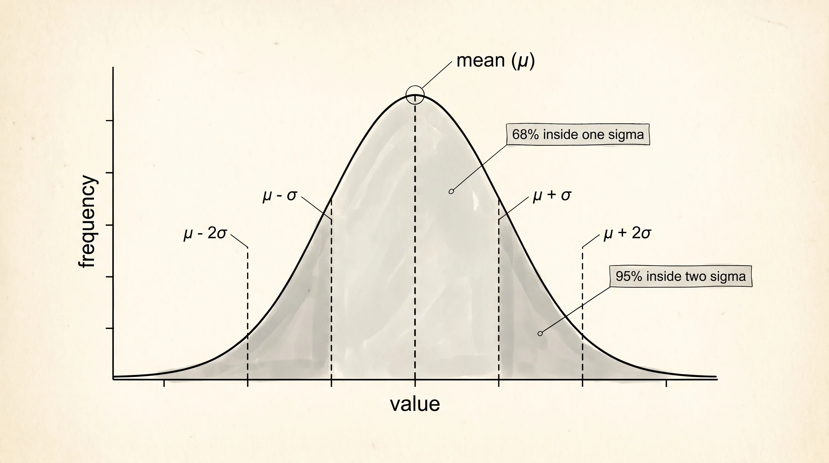
The standard deviation is the third squeeze and the most useful one once the first two are in your hand. It is the average distance from the mean — not the average of the numbers, but the average of how far each number sits from the mean. A small standard deviation means the days look like each other. A big standard deviation means the days swing wide. Two coffee carts with the same mean but different standard deviations are different businesses. The steady cart with the smaller deviation is the one you can plan around. The swinging cart with the bigger deviation needs a bigger cash buffer to survive a slow week.

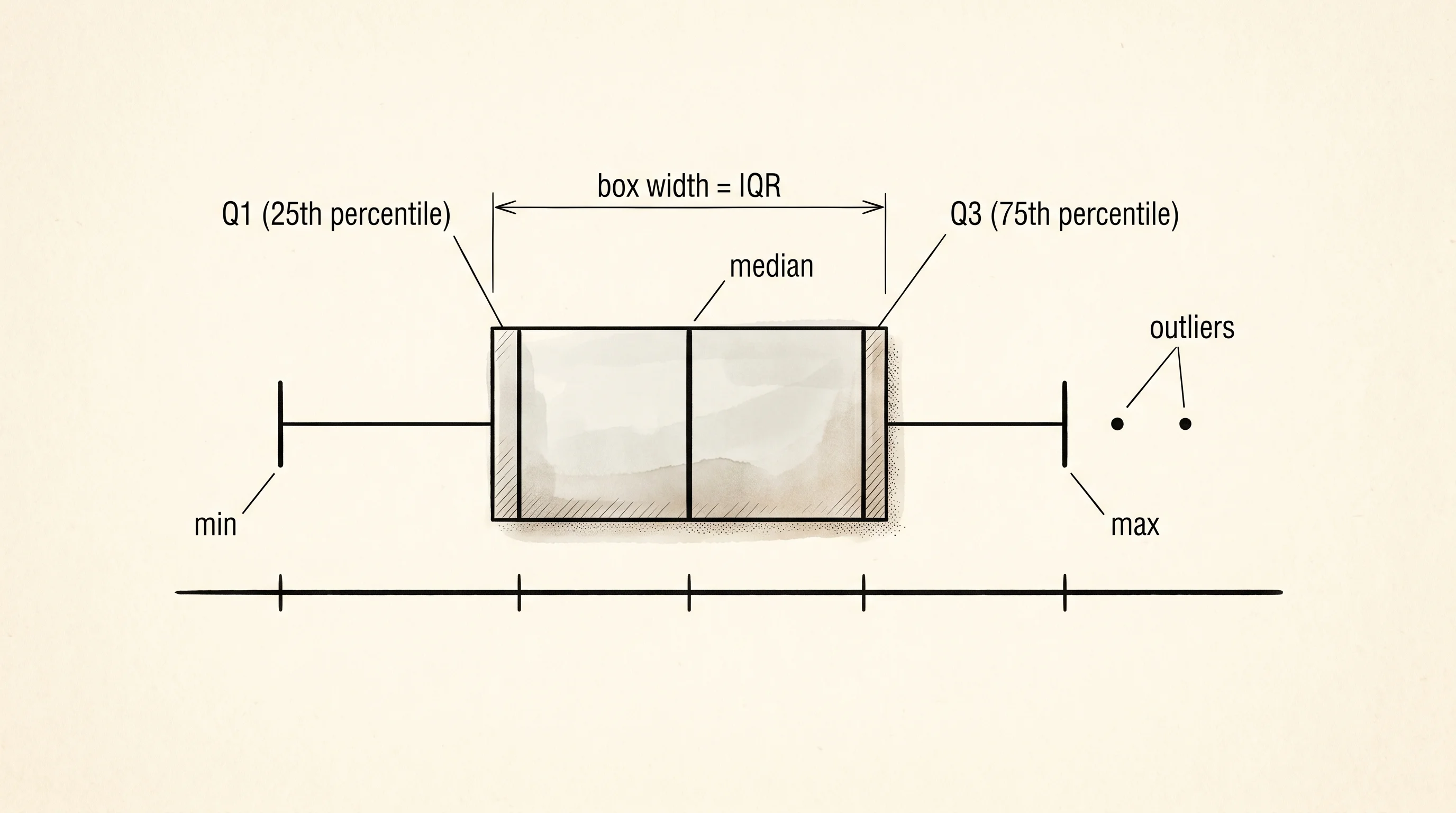
Min and max are the cheap ones — sort the list and take the ends. They are not the most informative numbers in the bag, but they tell you the worst day and the best day, and the gap between them sets the scale for everything else.

The interquartile range is the fifth number, and it is the one Tukey loved most. Sort the list and find the value a quarter of the way up — that is Q1, the first quartile. Find the value three quarters of the way up — that is Q3, the third quartile. The IQR is Q3 minus Q1, and it is the width of the middle half of the data. Half your days landed inside that range. Half landed outside. The IQR does the same job as the standard deviation but without letting one giant outlier blow up the answer, and Tukey's box plot uses it as the box.

Run the binary and watch the five numbers land for the cart.

--- five numbers that earn their keep ---
count    : 12
mean     : 249.3333
median   : 236.0000
std dev  : 56.9698
min      : 187.0000
max      : 410.0000
Q1       : 218.1250
Q3       : 257.8750
IQR      : 39.7500

--- old menu vs new menu (avg ticket size) ---
group A mean : 3.2500
group B mean : 3.7250
group A sd   : 0.1458
group B sd   : 0.1146
B beats A by : 14.62%

--- hours open vs cups sold ---
pearson r    : 0.9987
strength     : very strong

The mean is 249.33 dollars and the median is 236.00 dollars. The gap of 13 dollars is the freak day at 410 dragging the mean up while the median sits roughly where the typical day was. The standard deviation is 56.97, which feels big against a mean of 249 — and it is big because that one 410 day inflates the variance. The IQR is 39.75, much tighter, because it threw out the top and bottom quarter before measuring spread. One question worth asking — if the cart owner had to pick one number to report to his investor, which one would lie the least? The IQR and the median together, because they survive a freak day without telling a fiction about a normal week.

Once the five numbers are in your hand for one group, the second move is comparing two groups. The cart owner switches from his old menu to a new menu and wants to know whether the new menu actually sells more. He runs eight days on each menu and collects the average ticket size for each day. The simplest honest comparison is two means.

const GROUP_A: &[f64] = &[3.10, 3.40, 3.05, 3.25, 3.50, 3.20, 3.35, 3.15];
const GROUP_B: &[f64] = &[3.60, 3.80, 3.55, 3.90, 3.70, 3.65, 3.85, 3.75];

fn show_two_group_compare() {
    let ma = mean(GROUP_A);
    let mb = mean(GROUP_B);
    let lift_pct = (mb - ma) / ma * 100.0;
    println!("--- old menu vs new menu (avg ticket size) ---");
    println!("group A mean : {:.4}", ma);
    println!("group B mean : {:.4}", mb);
    println!("group A sd   : {:.4}", std_dev(GROUP_A));
    println!("group B sd   : {:.4}", std_dev(GROUP_B));
    println!("B beats A by : {:.2}%", lift_pct);
    println!();
}

The mean ticket on the old menu is 3.25 dollars and the mean ticket on the new menu is 3.73 dollars. The new menu beats the old one by 14.62 percent. That is the headline. But the standard deviations matter — the old menu has a spread of 0.15 dollars per day and the new menu has a spread of 0.11 dollars per day, both tight enough that the 14.62 percent gap is not noise. If the spreads had been ten times bigger, the same 48-cent difference would have been swallowed inside the day-to-day jitter and the cart owner would be fooling himself into a menu change that did nothing. The lesson is that comparing two means without checking the spreads is the same mistake Fisher's fertilizer trials taught the world to stop making 100 years ago.

The last move is correlation. The cart owner notices that he sold more cups on the days he stayed open longer, and he wants a single number that says how strongly hours and cups move together. Pearson's r is that number. It runs from negative 1 to positive 1. Plus 1 means perfect lock-step — every extra hour adds the same number of cups every time. Negative 1 means perfect opposition. Zero means no straight-line relationship at all.

const HOURS_OPEN: &[f64] = &[6.0, 7.0, 8.0, 9.0, 10.0, 11.0, 12.0];
const CUPS_SOLD: &[f64] = &[42.0, 55.0, 70.0, 88.0, 99.0, 118.0, 130.0];

fn pearson(xs: &[f64], ys: &[f64]) -> f64 {
    let mx = mean(xs);
    let my = mean(ys);
    let mut num = 0.0;
    let mut dx2 = 0.0;
    let mut dy2 = 0.0;
    for i in 0..xs.len() {
        let a = xs[i] - mx;
        let b = ys[i] - my;
        num += a * b;
        dx2 += a * a;
        dy2 += b * b;
    }
    num / (dx2.sqrt() * dy2.sqrt())
}

fn show_correlation() {
    let r = pearson(HOURS_OPEN, CUPS_SOLD);
    println!("--- hours open vs cups sold ---");
    println!("pearson r    : {:.4}", r);
    println!("strength     : {}", strength(r));
}

fn strength(r: f64) -> &'static str {
    let a = r.abs();
    if a >= 0.9 {
        "very strong"
    } else if a >= 0.7 {
        "strong"
    } else if a >= 0.4 {
        "moderate"
    } else {
        "weak"
    }
}

The math under the hood is simpler than the formula looks. For each day, take the distance from the mean of hours and the distance from the mean of cups. Multiply those two distances. Add up all twelve products. Divide by the product of the two standard deviations. The result is one number that summarizes whether the two columns move together. The cart's hours-and-cups correlation comes back at 0.9987 — basically lock-step, because the data was generated to be tight. A real cart's number would be lower, but the shape of the formula is the same.

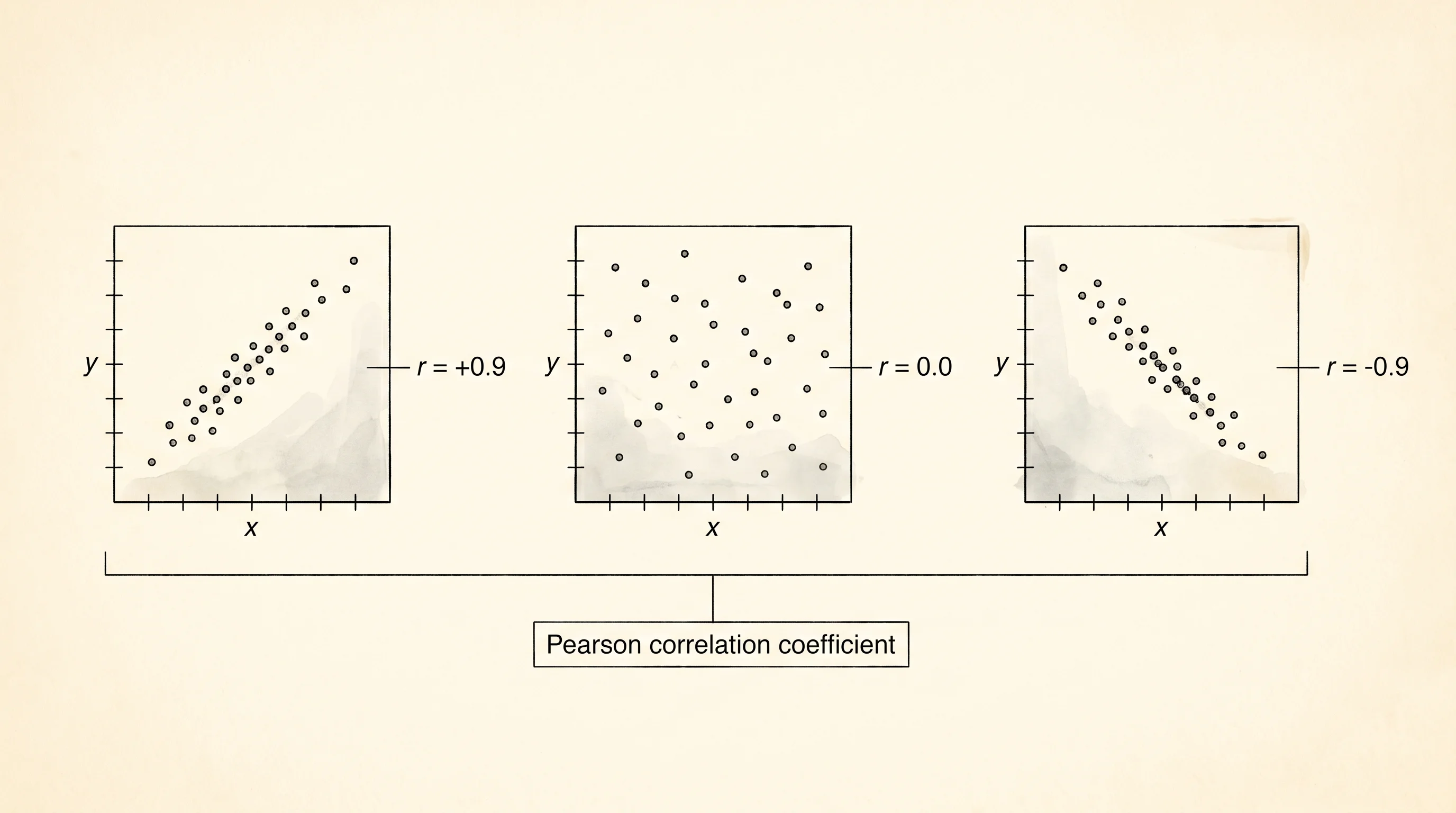
Pearson did the work on heredity data full of measurement error and human noise, and his coefficient still worked because it normalizes both columns by their own spread before comparing them. The trick is the normalization. Without it, a tall column and a short column would look uncorrelated even if they moved in perfect step, because the raw products would be tiny on one side and huge on the other. Dividing by the standard deviations puts both columns on the same scale, and the answer becomes a single dimensionless number anyone can read.

The thing none of these five numbers can do on its own is tell you whether tomorrow will look like today. Means and medians describe what happened. They do not extend forward in time, and a cart owner who needs to forecast next week's flour order needs a tool that reads the data as a sequence with a memory — which is what time-series analysis exists to solve.