Why CNNs Beat MLPs on Images
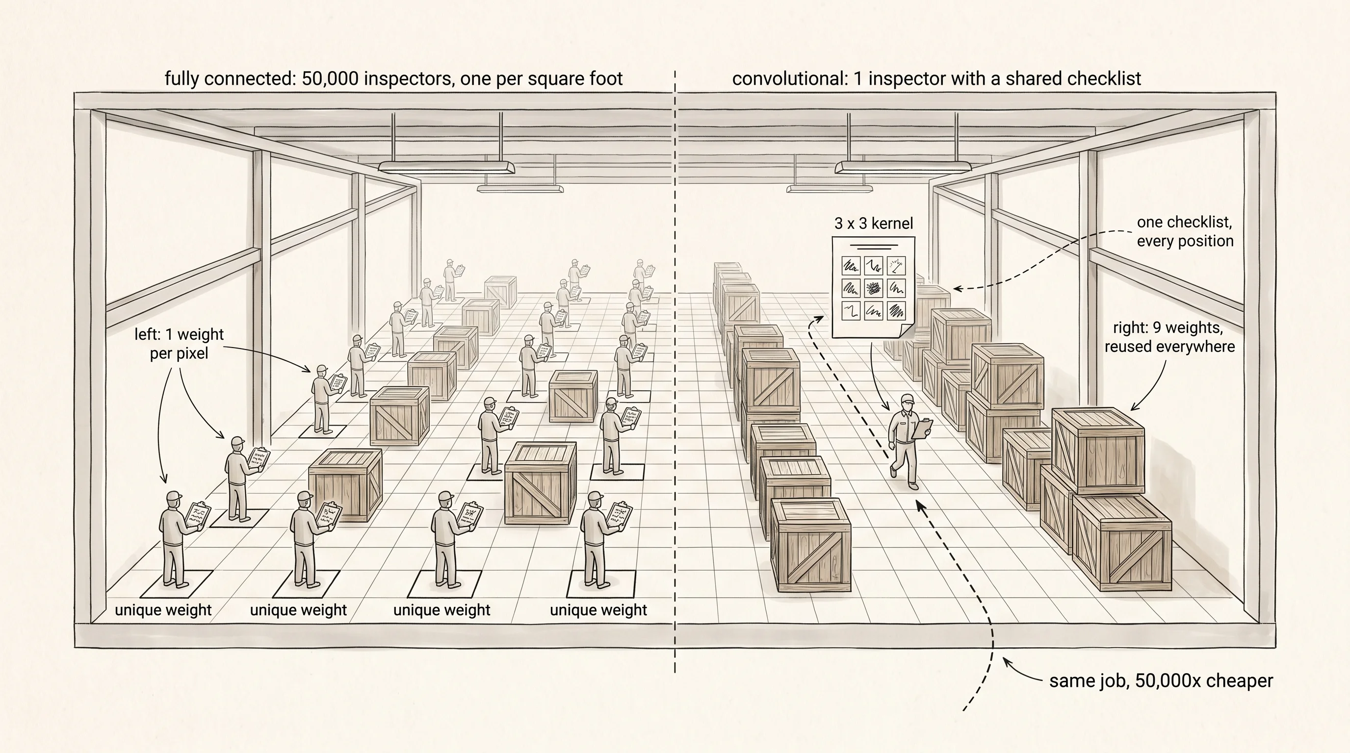
A brain that runs on numbers is finished. A brain that runs on pictures has not started. Imagine a warehouse the size of a city block. The owner needs every wooden crate inspected for a cracked plank. He goes to a hiring agency and gets two quotes. The first agency wants to hire 50,000 inspectors, one per square foot of floor, each one trained from zero on the kind of crack to look for. Whoever happens to be standing on the spot where a crate lands does the inspection. Every inspector is paid, every inspector is trained, every inspector knows nothing about cracks anywhere except the one square foot under his feet. The second agency wants to hire one inspector with a printed checklist. He walks the warehouse end to end, kneels at every crate, runs the same checklist down the same way, and goes home. Same job. One bill is 50,000 times the other. The first agency is a fully connected layer reading every pixel of an image. The second agency is a convolutional layer. The visual cortex you are about to build is the second agency.
The biology came first. In 1959 a Canadian neurosurgeon named David Hubel and a Swedish doctor named Torsten Wiesel were at Johns Hopkins trying to record what individual neurons in a cat's visual cortex actually did when the cat looked at something. They poked tungsten electrodes a fraction of a millimeter wide into the back of the cat's brain and held a card with a black dot in front of the cat's eye. Nothing fired. They moved the dot. Nothing fired. They got frustrated. Then a slide jammed sideways in their projector and a thin straight bar of light slid across the screen at an angle. The neuron erupted. They had stumbled on what they later called a simple cell — a neuron in the visual cortex that fires for an oriented edge at a small specific patch of the visual field. They published in 1962, kept working through the 1960s, and got the Nobel Prize in 1981. Their other discovery was the complex cell, which fires for an oriented edge anywhere within a larger patch — the position-tolerant version. The whole architecture of every image model in the world today is a software copy of what Hubel and Wiesel found by accident with a stuck slide.
The first person to take the biology and build it as code was Kunihiko Fukushima at NHK, the Japanese broadcasting company's research lab. In 1980 he wrote a paper called "Neocognitron" describing a layered network of small kernels that swept across an input image and pooled their outputs the way Hubel and Wiesel's complex cells pooled their simple cells. The kernels were not learned — Fukushima hand-tuned them. Yann LeCun at Bell Labs in 1989 was the first to take Fukushima's architecture and train the kernels with backpropagation. The result, LeNet, read handwritten zip codes off envelopes for the United States Postal Service. It worked, but training was slow, the data was small, and the rest of the field shrugged and went back to other methods. Convolutional networks sat in a side drawer for the next 23 years. Then in September 2012 a graduate student named Alex Krizhevsky, working with Ilya Sutskever and Geoffrey Hinton at the University of Toronto, took an 8-layer convolutional network, trained it on 1.2 million ImageNet photos using two consumer NVIDIA gaming GPUs sitting in his bedroom, and won the year's image recognition competition by 10 percentage points over the second-place team. The next year every entry in the same competition was a convolutional network. The current era of deep learning starts that week.
The job for the rest of this lesson is to feel why the conv version wins by building both and watching the parameter count collapse. Open edge_detector.py and start with the data. Eight rows by eight columns of binary pixels. Half the images contain a single full-height vertical line at a random column from 1 to 6. Half are pure noise — eight lit pixels scattered at random across the same grid. Both classes have the same number of lit pixels, so a detector cannot win by counting brightness.
import math
import random


GRID = 8
KERNEL = 3
FEATURE_MAP_SIZE = GRID - KERNEL + 1  # 6


def make_blank():
    return [[0 for _ in range(GRID)] for _ in range(GRID)]


def add_vertical_edge(image, col):
    for row in range(GRID):
        image[row][col] = 1


def add_speckle(image, rng, count):
    placed = 0
    while placed < count:
        r = rng.randint(0, GRID - 1)
        c = rng.randint(0, GRID - 1)
        if image[r][c] == 0:
            image[r][c] = 1
            placed += 1


def generate_edge_images(n, seed=0):
    rng = random.Random(seed)
    samples = []
    for index in range(n):
        image = make_blank()
        if index % 2 == 0:
            col = rng.randint(1, GRID - 2)
            add_vertical_edge(image, col)
            label = 1
        else:
            add_speckle(image, rng, count=GRID)
            label = 0
        samples.append((image, label))
    return samples
A vertical edge image looks like a single column of # cutting top to bottom. A noise image looks like eight # characters scattered like dropped coins. Eyeball them.
edge image (label = 1):       noise image (label = 0):
..#.....                      ......#.
..#.....                      ....#..#
..#.....                      ........
..#.....                      .#......
..#.....                      ........
..#.....                      ........
..#.....                      #..#....
..#.....                      ....#..#
Now the first detector — the 50,000-inspector agency. Flatten the 8 by 8 grid into a 64-element vector. Multiply by a 64-element weight vector. Add a bias. Run through a sigmoid. Every pixel position gets its own dedicated weight. Move the edge from column 3 to column 4 and the network sees a totally different input — none of the weights it learned for column-3-edge images apply to column-4-edge images.
def sigmoid(z):
    if z >= 0:
        return 1.0 / (1.0 + math.exp(-z))
    e = math.exp(z)
    return e / (1.0 + e)


def flatten(image):
    return [float(image[r][c]) for r in range(GRID) for c in range(GRID)]


class FullyConnectedDetector:
    def __init__(self, rng):
        self.weights = [rng.gauss(0.0, 0.1) for _ in range(GRID * GRID)]
        self.bias = 0.0

    def predict(self, image):
        z = self.bias
        for weight, value in zip(self.weights, flatten(image)):
            z += weight * value
        return sigmoid(z)
Sixty-four weights plus one bias. Sixty-five parameters in total. Now the second detector — the one inspector with a checklist. A single 3 by 3 window of nine weights. Slide that window across the image. At every position, multiply the nine kernel weights by the nine pixels under the window and sum. The result is a 6 by 6 feature map of activations — one number for every place the window could sit. Take the largest activation anywhere on the map. That single number is the detector's vote. The same nine weights are reused at every position. Move the edge from column 3 to column 4 and the kernel still finds it; its window walks past the new position and fires the same way.
class ConvolutionalDetector:
    def __init__(self, rng):
        self.kernel = [
            [rng.uniform(-0.3, 0.3) for _ in range(KERNEL)]
            for _ in range(KERNEL)
        ]
        self.bias = 0.0

    def feature_map(self, image):
        out = []
        for r in range(FEATURE_MAP_SIZE):
            row = []
            for c in range(FEATURE_MAP_SIZE):
                total = 0.0
                for kr in range(KERNEL):
                    for kc in range(KERNEL):
                        total += self.kernel[kr][kc] * image[r + kr][c + kc]
                row.append(total)
            out.append(row)
        return out

    def predict(self, image):
        fmap = self.feature_map(image)
        best = fmap[0][0]
        for row in fmap:
            for value in row:
                if value > best:
                    best = value
        return sigmoid(best + self.bias)
Nine weights plus one bias. Ten parameters. Six and a half times fewer than the fully connected detector — and that ratio explodes the moment the image gets bigger. A 224 by 224 image (the standard ImageNet input) gives the fully connected detector 50,176 weights for a single output neuron. The convolutional detector still has nine. The ratio is over 5000.
Both detectors need a way to learn. We have not built backprop through convolution yet, so use the same finite-difference trick from the manual backprop lesson. Wiggle each parameter up by a tiny epsilon, measure the loss, wiggle it down by the same epsilon, measure again, divide by 2 epsilon. The result is a numerical estimate of the gradient — the same answer the analytical formula would give, just slower. Apply it to every parameter in turn, then update everyone at once.
def binary_cross_entropy(prediction, target):
    epsilon = 1e-12
    p = min(max(prediction, epsilon), 1.0 - epsilon)
    return -(target * math.log(p) + (1 - target) * math.log(1.0 - p))


def loss_on(detector, samples):
    total = 0.0
    for image, label in samples:
        total += binary_cross_entropy(detector.predict(image), label)
    return total / len(samples)


def train_conv(detector, samples, epochs, learning_rate, epsilon=1e-2):
    for _ in range(epochs):
        kernel_grads = [[0.0] * KERNEL for _ in range(KERNEL)]
        for r in range(KERNEL):
            for c in range(KERNEL):
                original = detector.kernel[r][c]
                detector.kernel[r][c] = original + epsilon
                up = loss_on(detector, samples)
                detector.kernel[r][c] = original - epsilon
                down = loss_on(detector, samples)
                detector.kernel[r][c] = original
                kernel_grads[r][c] = (up - down) / (2 * epsilon)
        original_bias = detector.bias
        detector.bias = original_bias + epsilon
        up = loss_on(detector, samples)
        detector.bias = original_bias - epsilon
        down = loss_on(detector, samples)
        detector.bias = original_bias
        bias_grad = (up - down) / (2 * epsilon)
        for r in range(KERNEL):
            for c in range(KERNEL):
                detector.kernel[r][c] -= learning_rate * kernel_grads[r][c]
        detector.bias -= learning_rate * bias_grad
The fully connected version is the same code with a longer inner loop — 64 weights instead of nine. Train both detectors on 80 images and watch what each one learns.
train_samples = generate_edge_images(80, seed=1)

fc = FullyConnectedDetector(random.Random(0))
conv = ConvolutionalDetector(random.Random(0))

train_fc(fc, train_samples, epochs=80, learning_rate=3.0)
train_conv(conv, train_samples, epochs=400, learning_rate=1.0)

print("FC detector — 64 weights laid out as the 8x8 grid they read:")
for r in range(GRID):
    cells = [f"{fc.weights[r * GRID + c]:+5.2f}" for c in range(GRID)]
    print(" ".join(cells))

print("\nconv detector — the 3x3 kernel reused at every position:")
for r in range(KERNEL):
    cells = [f"{conv.kernel[r][c]:+5.2f}" for c in range(KERNEL)]
    print(" ".join(cells))
Print and stare.
FC detector — 64 weights laid out as the 8x8 grid they read:
-1.57 +0.83 +1.05 +0.60 +1.37 +0.46 +0.74 -1.80
-1.58 +1.67 +1.15 +1.75 +0.01 +0.14 +0.18 -2.17
-2.40 -0.29 -0.34 +0.46 +0.44 +1.58 +1.52 -1.24
-1.67 +1.94 +1.14 -0.05 -1.03 +0.74 -1.56 -1.15
-1.76 -0.17 +0.10 -0.45 -0.11 -0.28 +0.49 -1.30
-1.90 -0.45 +0.98 +1.17 +0.47 +1.81 -0.78 -2.50
-1.76 -0.78 -0.23 -0.43 +1.46 -0.44 +0.42 -0.25
-2.35 +0.55 -0.02 +0.71 +0.78 +0.00 +1.06 -0.79
conv detector — the 3x3 kernel reused at every position:
+2.35 -2.80 -2.06
+2.36 -1.84 -2.06
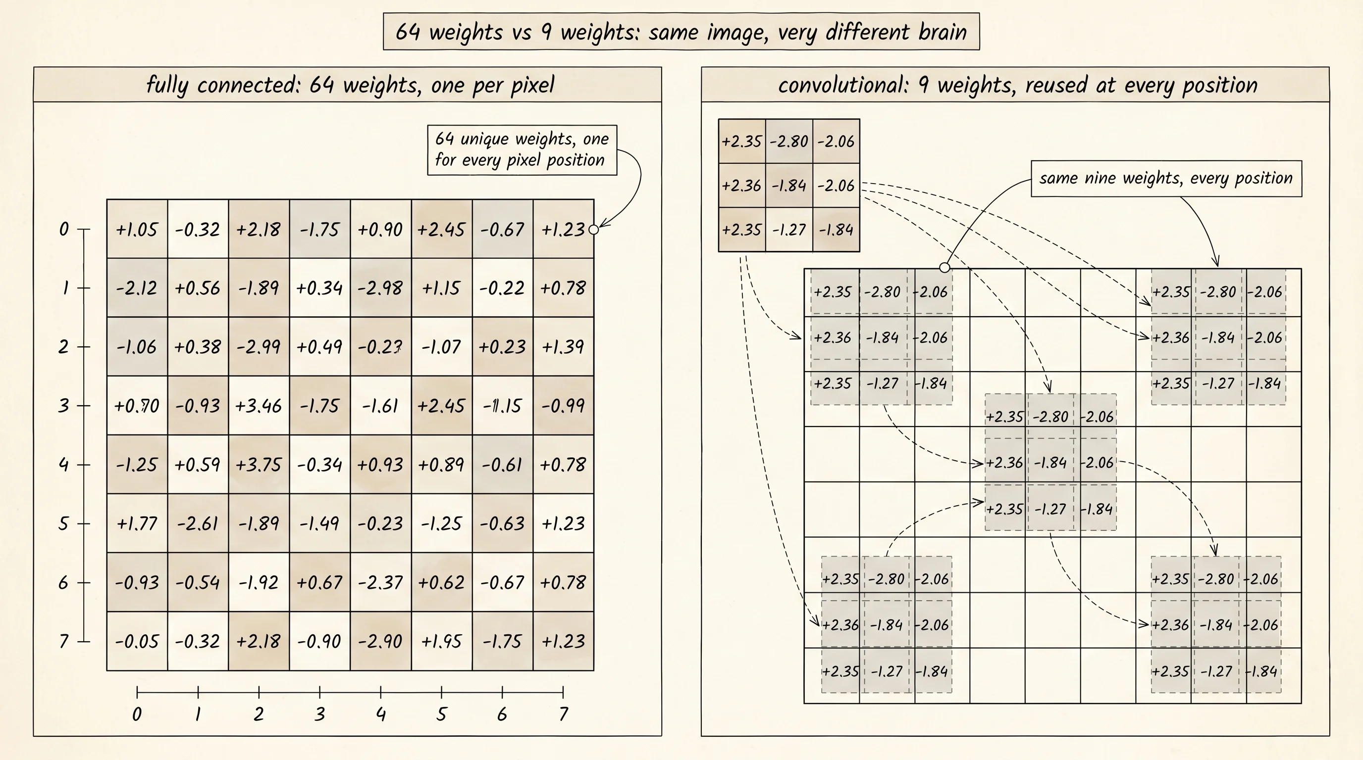
+2.35 -1.27 -1.84The 8 by 8 grid on top is a wall of numbers. Some columns lean negative, some lean positive, but there is no clean repeating pattern — the network has memorized 80 specific images and chosen a number for every pixel position. The 3 by 3 grid on the bottom is something else. Every entry on the left column is between +2.35 and +2.36. Every entry on the middle and right columns is negative. The kernel says "fire when there is a lit pixel on my left and dark pixels to my right." That is the textbook definition of a vertical edge detector, and the same kernel that signal-processing engineers have hand-designed since the 1960s under the name Sobel filter. Nine random numbers walked into training and a Sobel filter walked out. Nobody told the network what an edge looked like.
A small question. The fully connected detector hits 100% accuracy on its training images. The convolutional detector only hits 95%. Which one is the better detector? Run both on a fresh batch of 40 images the network has never seen. The fully connected detector drops to 80% on the new set. The convolutional detector holds at 87.5%. The fully connected detector won the practice exam by memorizing every photo on the answer key. The convolutional detector won the real exam by learning what an edge actually looks like — the same vertical bar, anywhere on the grid, no matter what column it sits in. Six and a half times fewer parameters. Better generalization. This is the move that started the modern era.
Convolutions slide across the image, but watch what happens at the borders.