Backprop By Hand
A car runs on a thousand small explosions a minute and most of the people who drive one have never opened the hood. The engineer who has — the one who pulled the head off, slid the cylinders out, scraped the carbon ring on each piston, and laid the timing chain across the bench in the order it came off — is the only one in the room who is no longer impressed by the magic. The autograd engine from the last lesson is the same kind of magic. Call .backward() and the gradient appears at every weight. The loss drops on the next step. Nobody asks where the numbers came from. Rebuild the engine on the garage floor once. Pick a tiny network with hard-coded weights, run one input through it by hand, walk the chain rule backwards by hand, write each gradient down on paper as you go, and then check every paper number against a finite-difference estimate. Do that one time and the autograd magic stops being magic.
David Rumelhart, Geoffrey Hinton, and Ronald Williams put backprop in the hands of every neural network researcher in 1986 with a 4-page note in Nature called Learning representations by back-propagating errors. The algorithm itself was older — Seppo Linnainmaa had written down reverse-mode differentiation in 1970, and Paul Werbos had applied it to neural networks in his 1974 PhD thesis — but it was the Rumelhart paper that finally got read. The paper showed that a 2-layer network of sigmoid neurons trained by backpropagating the squared error could solve XOR, learn to pronounce English text, and recognize family relationships in a tiny made-up dataset. Within 5 years the algorithm was in every textbook. Forty years later Andrej Karpathy, by then Director of AI at Tesla, posted an exercise on his blog called Becoming a Backprop Ninja — derive every gradient in a small network by hand, no autograd, no shortcuts. The exercise sounds tedious until you notice who finishes it. The engineers who later wrote FlashAttention, the GPU kernels that quadrupled training speed for every transformer, and the people who hand-tune low-level CUDA inside Anthropic and OpenAI all learned backprop the way you are about to: with a pen, a small network, and the chain rule applied one node at a time.
The network is the smallest one you can still call a network: 2 inputs, 3 hidden neurons with ReLU, 2 output neurons with softmax, cross-entropy loss against a one-hot target. Weights are not random. Every weight is a number you pick and write down once, so the forward pass and the backward pass print the same numbers every time anyone runs the file. Open gradient_trace.py and write the network as a dictionary keyed by name.
def build_network():
    return {
        "W1": [[ 0.10, -0.20],
               [ 0.30,  0.40],
               [-0.20,  0.50]],
        "b1": [ 0.05, -0.10,  0.20],
        "W2": [[ 0.20, -0.30,  0.10],
               [-0.10,  0.40,  0.20]],
        "b2": [ 0.10, -0.05],
    }

INPUT  = [0.5, 0.8]
TARGET = [1.0, 0.0]
Read the shapes. W1 is 3 rows by 2 columns: 3 hidden neurons each looking at 2 inputs. W2 is 2 rows by 3 columns: 2 output neurons each looking at 3 hidden activations. The biases match the row counts. The input is a single point. The target says class 0 is the right answer. 17 numbers go into the network and 17 gradients should come out at the end — one per weight, one per bias.
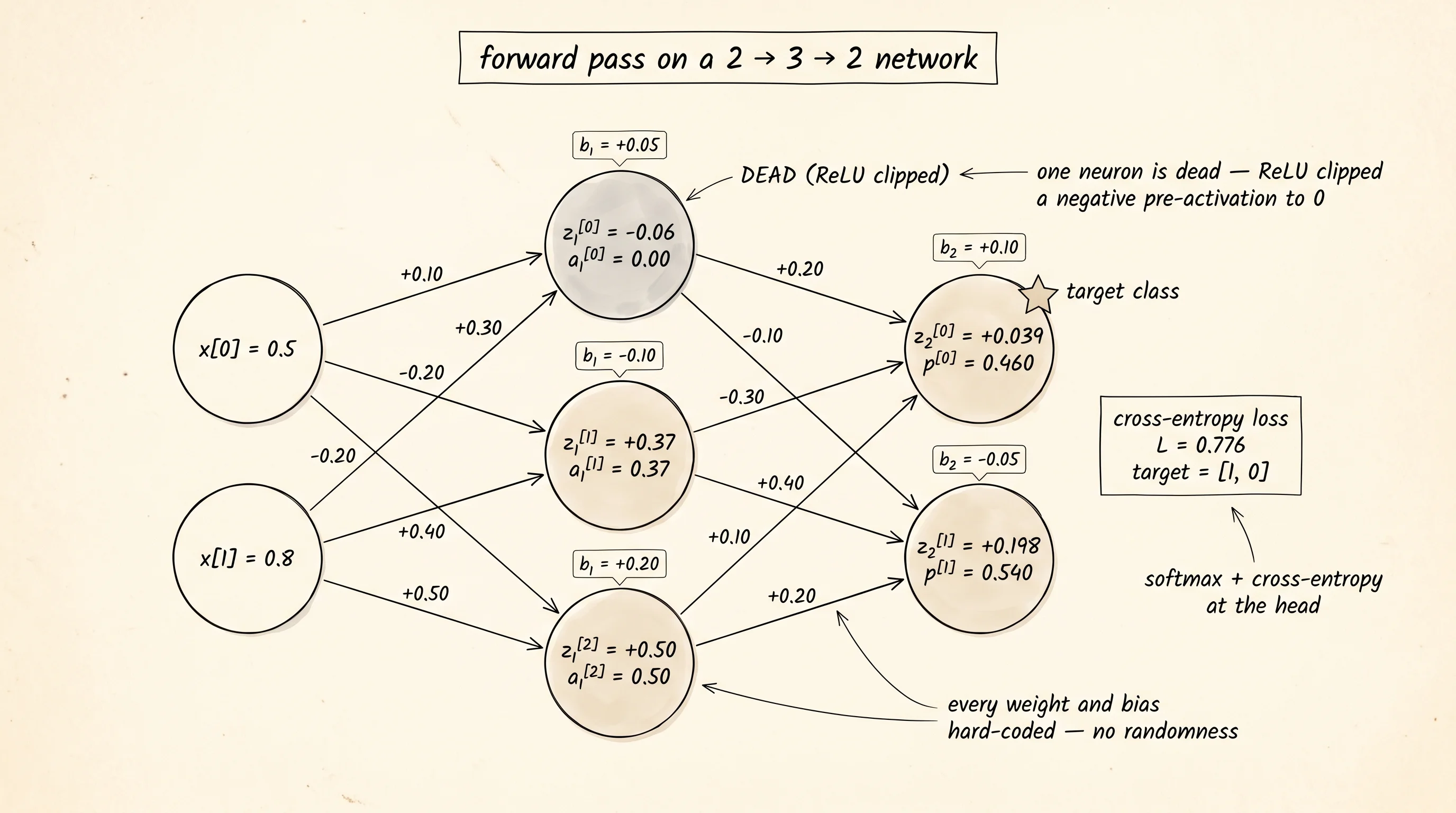
The forward pass is a list of small computations stacked on top of each other. Multiply the input by W1 row by row, add b1, take ReLU. Multiply the result by W2 row by row, add b2, take softmax. Compare the softmax output to the target with cross-entropy. The function forward_trace runs all of that and prints every multiply, every add, every activation, the softmax, and the loss. Run the project and the first half of the trace looks like this:
input    x = [0.5000, 0.8000]
target   t = [1, 0]  (class 0)

hidden pre-activations  z1 = W1 @ x + b1
  z1[0] = +0.0500 + (+0.1000 * +0.5000) + (-0.2000 * +0.8000) = -0.060000
  z1[1] = -0.1000 + (+0.3000 * +0.5000) + (+0.4000 * +0.8000) = +0.370000
  z1[2] = +0.2000 + (-0.2000 * +0.5000) + (+0.5000 * +0.8000) = +0.500000

hidden activations  a1 = relu(z1)
  a1[0] = relu(-0.060000) = 0.000000   [DEAD (clipped to 0)]
  a1[1] = relu(+0.370000) = 0.370000   [passes]
  a1[2] = relu(+0.500000) = 0.500000   [passes]

output pre-activations  z2 = W2 @ a1 + b2
  z2[0] = +0.1000 + (+0.2000 * +0.0000) + (-0.3000 * +0.3700) + (+0.1000 * +0.5000) = +0.039000
  z2[1] = -0.0500 + (-0.1000 * +0.0000) + (+0.4000 * +0.3700) + (+0.2000 * +0.5000) = +0.198000

softmax  p = softmax(z2)
  p[0] = 0.460334
  p[1] = 0.539666

cross-entropy loss  L = -sum(t * log(p))
  L = 0.775804
The first hidden neuron came out negative. ReLU clipped it to 0. That dead neuron is the most useful number on the page. Whatever gradient flows back into hidden neuron 0 from the output layer, ReLU's derivative is 0 there, and so the gradient gets blocked at that gate. Both weights into that neuron and its bias will receive a gradient of exactly 0 from this single training example. Gradient gating by ReLU is one of the things autograd does silently. Doing it by hand makes you see it.
The output layer says class 0 with probability 0.460 and class 1 with probability 0.540 — the network thinks the wrong answer is slightly more likely. Cross-entropy of 0.776 measures the surprise. Now the engine work starts: every weight and every bias gets a gradient that says "if I nudge you by a tiny amount, this is how much the loss will change." The chain rule applied to the computational graph gives every one of those numbers exactly.
The chain rule is the rule for stacked functions. If a value c depends on a value b and b depends on a value a, then a small change in a produces a change in c equal to the change in b per unit change in a times the change in c per unit change in b. Written as derivatives: dc/da = (dc/db) · (db/da). The neural network is one giant stacked function. The loss depends on the output probabilities, which depend on the output pre-activations, which depend on the hidden activations, which depend on the hidden pre-activations, which depend on the inputs and weights. To get the gradient of the loss with respect to a weight near the input, walk that chain from the loss back to the weight, multiplying local derivatives as you go.
Backprop is the chain rule applied to the graph in reverse, with one trick that makes it tractable. Carry one number per node — the gradient of the loss with respect to that node's value. Compute it once. Use it to feed every parent of that node. Never recompute the same partial product twice. The backward pass walks the same nodes the forward pass walked, but in reverse, and at every node it multiplies the upstream gradient by the local derivative.
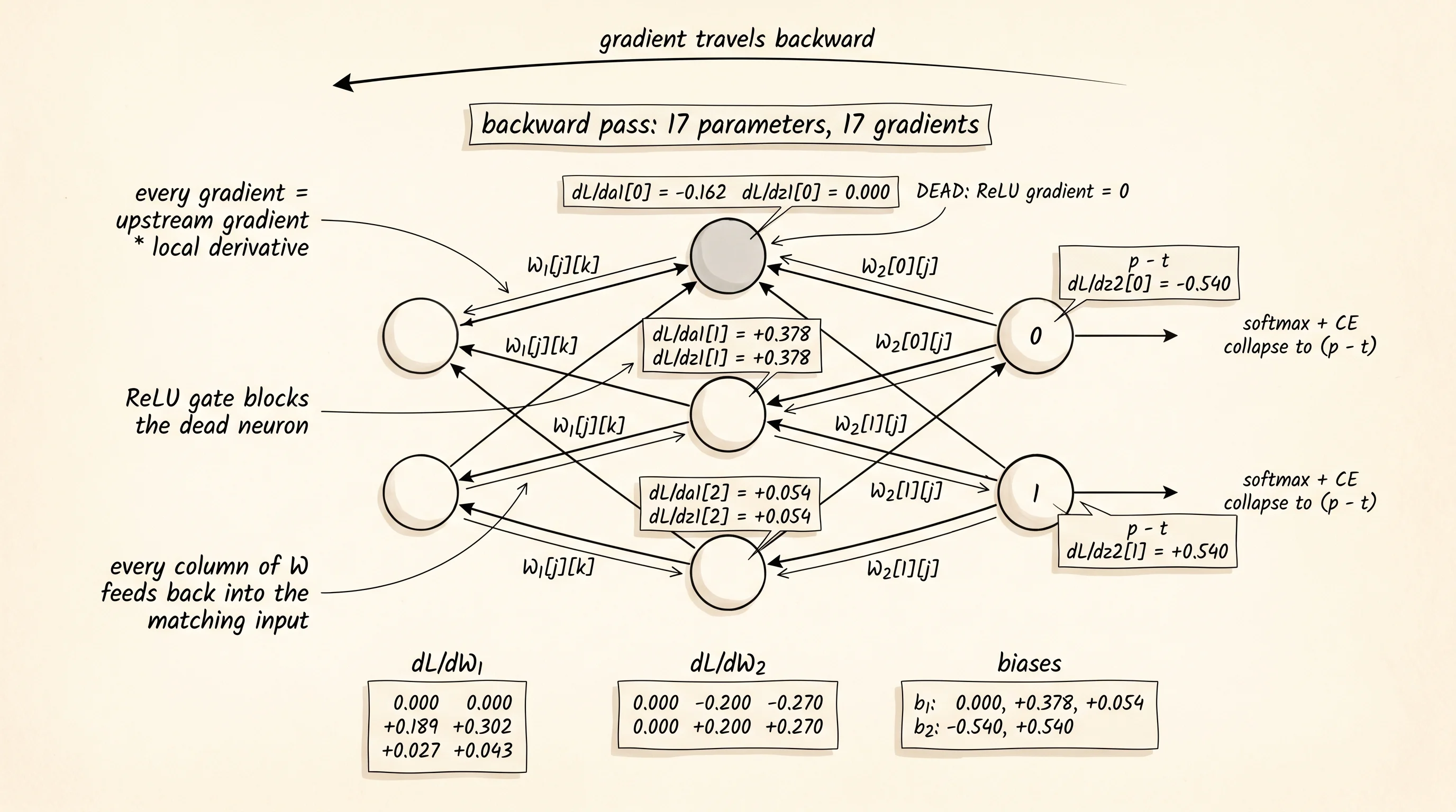
Start at the loss. The first non-trivial gradient is dL/dz2 — the gradient of the loss with respect to the output pre-activations. Cross-entropy on top of softmax gives the cleanest result in the entire algorithm: dL/dz2 = p − t. The probabilities minus the one-hot target. No exponentials. No logs. One subtraction per output neuron. The derivation of why this happens lives in the categorical-cross-entropy lesson; the magic trick is that the messy softmax derivative and the messy log derivative cancel each other when you compose them.
step 1: dL/dz2 from softmax + cross-entropy collapse to (p - t)
  dL/dz2[0] = p[0] - t[0] = 0.460334 - 1 = -0.539666
  dL/dz2[1] = p[1] - t[1] = 0.539666 - 0 = +0.539666
The output for class 0 is too low so its pre-activation needs to push up — the gradient is negative, which under gradient descent means subtract a negative, which means add. The output for class 1 is too high and its gradient says push down. Two numbers. Every gradient downstream of the loss comes from these two.
The bias on the output layer adds 1 unit of itself per unit of pre-activation. dz2/db2 = 1. So dL/db2 = dL/dz2 directly. The weights are the interesting case. Each weight W2[i][j] multiplies the hidden activation a1[j] to produce the output pre-activation z2[i]. The local derivative of z2[i] with respect to W2[i][j] is just a1[j]. Multiply that by the upstream gradient dL/dz2[i] and you have dL/dW2[i][j].
step 3: dL/dW2[i][j] = dL/dz2[i] * a1[j]
  dL/dW2[0][1] = dL/dz2[0] * a1[1] = -0.539666 * 0.370000 = -0.199677
  dL/dW2[0][2] = dL/dz2[0] * a1[2] = -0.539666 * 0.500000 = -0.269833
  dL/dW2[1][1] = dL/dz2[1] * a1[1] = +0.539666 * 0.370000 = +0.199677
  dL/dW2[1][2] = dL/dz2[1] * a1[2] = +0.539666 * 0.500000 = +0.269833
Two gradients on the W2 row pointing at hidden neuron 0 are exactly 0 because a1[0] is exactly 0. The dead ReLU is already showing up. The other 4 weights get gradients with the same magnitudes mirrored across the two output rows because the upstream gradients on the two outputs are negatives of each other.
Now the gradient has to travel from the output pre-activations back through the hidden activations. Every hidden neuron a1[j] feeds both output neurons. So the change in the loss caused by nudging a1[j] picks up contributions from both output paths: dL/da1[j] = sum over i of dL/dz2[i] · W2[i][j]. The same multiplication you used in the forward pass, but with the gradient flowing the other direction.
step 4: dL/da1[j] = sum_i  dL/dz2[i] * W2[i][j]
  dL/da1[0] = (-0.539666 * +0.2000) + (+0.539666 * -0.1000) = -0.161900
  dL/da1[1] = (-0.539666 * -0.3000) + (+0.539666 * +0.4000) = +0.377767
  dL/da1[2] = (-0.539666 * +0.1000) + (+0.539666 * +0.2000) = +0.053967
The forward pass took inputs and pushed them through W2 to get outputs. The backward pass takes output gradients and pulls them through the same W2 to get input gradients. Same matrix, opposite direction. Every backprop implementation in every framework, from PyTorch to JAX to MLX, does exactly this transpose-and-multiply at the linear-layer level.
The hidden activation a1[j] came from ReLU(z1[j]). ReLU's derivative is 1 if z1[j] was positive and 0 if it was negative. Multiply dL/da1[j] by that gate to get dL/dz1[j].
step 5: dL/dz1[j] = dL/da1[j] * relu'(z1[j])
  dL/dz1[0] = -0.161900 * 0 = -0.000000   [DEAD: gradient blocked]
  dL/dz1[1] = +0.377767 * 1 = +0.377767   [alive]
  dL/dz1[2] = +0.053967 * 1 = +0.053967   [alive]
The dead neuron stops the gradient cold. The two live neurons pass it through unchanged. ReLU's contribution to backprop is a single multiply by either 1 or 0, decided per neuron, per example, by which side of zero its pre-activation landed on during the forward pass.
The last two gradients fall out the same way the W2 gradients did. dL/db1 = dL/dz1 because the bias adds 1 per unit. dL/dW1[j][k] = dL/dz1[j] · x[k] because the weight multiplies the input.
step 7: dL/dW1[j][k] = dL/dz1[j] * x[k]
  dL/dW1[0][0] = dL/dz1[0] * x[0] = -0.000000 * +0.5000 = -0.000000
  dL/dW1[1][0] = dL/dz1[1] * x[0] = +0.377767 * +0.5000 = +0.188883
  dL/dW1[1][1] = dL/dz1[1] * x[1] = +0.377767 * +0.8000 = +0.302213
  dL/dW1[2][0] = dL/dz1[2] * x[0] = +0.053967 * +0.5000 = +0.026983
  dL/dW1[2][1] = dL/dz1[2] * x[1] = +0.053967 * +0.8000 = +0.043173
Every weight, every bias, every gradient. 17 parameters in, 17 gradients out. The whole derivation is 7 steps of multiplying upstream gradients by local derivatives, walking from the loss back to the input. Nothing else.
The reasonable next thought is "how do I know any of these numbers are right?" The answer is finite differences. Pick one parameter, bump it up by a tiny amount h, recompute the loss, bump it down by h, recompute the loss, and divide the difference by 2h. That number is the central-difference estimate of the gradient. It is the definition of the derivative computed empirically. If your analytical gradient and your finite-difference estimate disagree, the analytical derivation is wrong.
def verify_gradient(network, inputs, target, param_name, indices, h=1e-5):
    parameter = network[param_name]
    if len(indices) == 1:
        (j,) = indices
        original = parameter[j]
        parameter[j] = original + h
        loss_plus  = loss_at(network, inputs, target)
        parameter[j] = original - h
        loss_minus = loss_at(network, inputs, target)
        parameter[j] = original
    else:
        i, j = indices
        original = parameter[i][j]
        parameter[i][j] = original + h
        loss_plus  = loss_at(network, inputs, target)
        parameter[i][j] = original - h
        loss_minus = loss_at(network, inputs, target)
        parameter[i][j] = original
    return (loss_plus - loss_minus) / (2.0 * h)
Run that on every one of the 17 parameters. Print a table with the parameter name, the analytical gradient, the finite-difference estimate, the absolute difference, and a yes/no for whether they match to 6 decimal places.
parameter           analytical     finite-diff         |delta|     match
------------------------------------------------------------------------
W1[0][0]             -0.000000       +0.000000        0.00e+00       yes
W1[0][1]             -0.000000       +0.000000        0.00e+00       yes
W1[1][0]             +0.188883       +0.188883        4.12e-12       yes
W1[1][1]             +0.302213       +0.302213        2.29e-12       yes
W1[2][0]             +0.026983       +0.026983        5.89e-13       yes
W1[2][1]             +0.043173       +0.043173        3.50e-12       yes
b1[0]                -0.000000       +0.000000        0.00e+00       yes
b1[1]                +0.377767       +0.377767        2.86e-12       yes
b1[2]                +0.053967       +0.053967        6.73e-12       yes
W2[0][0]             -0.000000       +0.000000        0.00e+00       yes
W2[0][1]             -0.199677       -0.199677        3.25e-12       yes
W2[0][2]             -0.269833       -0.269833        3.36e-13       yes
W2[1][0]             +0.000000       +0.000000        0.00e+00       yes
W2[1][1]             +0.199677       +0.199677        3.25e-12       yes
W2[1][2]             +0.269833       +0.269833        5.21e-12       yes
b2[0]                -0.539666       -0.539666        4.88e-12       yes
b2[1]                +0.539666       +0.539666        4.88e-12       yes
Every row matches to 6 decimal places. The largest disagreement is 7 picounits — the rounding error left over from doing arithmetic on 64-bit floats. Two completely different methods of computing the same gradient agree to a part in ten billion. The analytical derivation is right. The chain rule worked. The engine is rebuilt and there is no magic left in it. Every line of PyTorch's loss.backward() does this same walk through this same shape of nodes, multiplying upstream gradients by local derivatives. The only difference is that PyTorch tracks the graph for you, and that the graph it tracks has hundreds of millions of nodes instead of 17.
A small question. Why does the central difference match the analytical gradient to 12 decimal places when the function does only 1 forward pass through 17 parameters? Because the central-difference formula is set up so the linear error in h cancels. The forward difference (loss_plus − loss_at_origin) / h leaves an error proportional to h. The central difference (loss_plus − loss_minus) / (2h) cancels that linear term and leaves only an error proportional to h². At h = 1e-5 that error is around 1e-10, which is exactly the residual the table shows. Pick h too large and the error grows; pick h too small and floating-point cancellation in the numerator destroys the result. The sweet spot for double precision is around 1e-5 to 1e-7, which is why the project hard-codes h = 1e-5.
You can train a brain on numbers, but real data — images, audio, text — has structure the brain has to be built around.