Tape-Based Autograd

A flight recorder sits in the tail of every commercial jet. While the plane flies, the recorder logs every input the pilot touches and every output the engines produce. After the flight, an investigator plays the tape back and reads the story. Autograd is a flight recorder for math. While the network runs forward, every multiply and add and exponential gets logged onto a tape with a note about its inputs. After the loss comes out the other end, the tape gets played in reverse, and at every recorded step the chain rule turns into a tiny piece of arithmetic. By the time the tape rewinds to the start, every weight has a gradient sitting next to it. No finite differences. No symbolic algebra. Just record and replay.

The first person to write this down was a Stanford engineer named Robert Wengert. In 1964 he published a four-page paper called A simple automatic derivative evaluation program. His idea was forward-mode AD: walk forward through the expression, and at every operation, carry along not just the value but also its derivative with respect to one chosen input. Six years later a Finnish master's student named Seppo Linnainmaa noticed that forward-mode is wasteful when you have many inputs and one output, which is exactly the shape of every loss function. His fix, written into his 1970 thesis, was reverse-mode AD: do the forward pass first, store everything, then walk backward and compute the gradient of the output with respect to every input at the same time. The math is identical to backpropagation, the algorithm Rumelhart and Hinton would later make famous, except Linnainmaa wrote it down 16 years earlier and almost nobody read it. The idea sat untouched for 40 years until a research group at the University of Montreal led by Yoshua Bengio shipped Theano in 2010 — the first practical autograd built into a real deep learning library. Theano traced a static graph and compiled it ahead of time, which was fast but rigid. In 2017 a small team at Facebook released PyTorch with a different choice: build the tape on the fly, every forward pass. That dynamic graph made the library feel like normal Python — write a for loop, autograd records every iteration — and within two years it had taken the framework war.

To build this from scratch you need one class. Call it Value. A Value carries four things: the actual number it stores (data), the gradient of the final output with respect to it (grad, starts at zero), a function that knows how to push the gradient back through the operation that produced it (_backward), and the set of Value objects that fed into its creation (_prev). The forward operations on Value get wired to Python's operator slots — plus, times, power, exponential — so a normal-looking math expression silently builds a graph as it executes. Open a file called engine.py and start typing.

import math
 
 
class Value:
    def __init__(self, data, _children=(), _op=""):
        self.data = data
        self.grad = 0.0
        self._backward = lambda: None
        self._prev = set(_children)
        self._op = _op
 
    def __repr__(self):
        return f"Value(data={self.data:.4f}, grad={self.grad:.4f})"

A bare Value does nothing. Add the first operation, __add__, and the structure of every other operation falls out of it. Three things have to happen inside the operator. Build a new Value that holds the sum. Define a _backward closure that knows the local derivative of addition (which is 1 for both inputs) and uses it to add the upstream gradient onto each child. Attach the closure and the parents to the new Value and return it.

    def __add__(self, other):
        other = other if isinstance(other, Value) else Value(other)
        out = Value(self.data + other.data, (self, other), "+")
 
        def _backward():
            self.grad += out.grad
            other.grad += out.grad
 
        out._backward = _backward
        return out

The += matters. The same Value can feed into many operations, and the chain rule sums gradient contributions from every path. Overwrite instead of accumulate and the gradient on a shared variable will be wrong every time. Multiplication uses the product rule.

    def __mul__(self, other):
        other = other if isinstance(other, Value) else Value(other)
        out = Value(self.data * other.data, (self, other), "*")
 
        def _backward():
            self.grad += other.data * out.grad
            other.grad += self.data * out.grad
 
        out._backward = _backward
        return out

d(a*b)/da = b and d(a*b)/db = a. The closure captures self.data and other.data from the forward pass and uses them at backward time. This is why we need a tape — the forward values are inputs to the backward pass, and a recorder is the cleanest way to hold onto them. Power, negation, exponential, and log follow the same shape, each with its own one-line derivative.

    def __pow__(self, exponent):
        assert isinstance(exponent, (int, float))
        out = Value(self.data ** exponent, (self,), f"**{exponent}")
 
        def _backward():
            self.grad += exponent * (self.data ** (exponent - 1)) * out.grad
 
        out._backward = _backward
        return out
 
    def __neg__(self):
        return self * -1
 
    def exp(self):
        out = Value(math.exp(self.data), (self,), "exp")
 
        def _backward():
            self.grad += out.data * out.grad
 
        out._backward = _backward
        return out
 
    def log(self):
        out = Value(math.log(self.data), (self,), "log")
 
        def _backward():
            self.grad += (1.0 / self.data) * out.grad
 
        out._backward = _backward
        return out

The activations follow the same pattern. ReLU passes the gradient straight through if the input was positive and zeros it out otherwise. Sigmoid's derivative is s * (1 - s) where s is the output, which the closure already has. Tanh's derivative is 1 - t**2, again pulled from the output.

    def relu(self):
        out = Value(self.data if self.data > 0.0 else 0.0, (self,), "relu")
 
        def _backward():
            self.grad += (1.0 if self.data > 0.0 else 0.0) * out.grad
 
        out._backward = _backward
        return out
 
    def sigmoid(self):
        s = 1.0 / (1.0 + math.exp(-self.data))
        out = Value(s, (self,), "sigmoid")
 
        def _backward():
            self.grad += s * (1.0 - s) * out.grad
 
        out._backward = _backward
        return out
 
    def tanh(self):
        t = math.tanh(self.data)
        out = Value(t, (self,), "tanh")
 
        def _backward():
            self.grad += (1.0 - t * t) * out.grad
 
        out._backward = _backward
        return out

Two reverse operators round out the math grammar. Subtraction is addition of a negative. Division is multiplication by a power of -1. Adding __radd__ and __rmul__ lets 2 + x work the same as x + 2.

    def __sub__(self, other):
        return self + (-other)
 
    def __truediv__(self, other):
        return self * (other ** -1 if isinstance(other, Value) else Value(other) ** -1)
 
    def __radd__(self, other):
        return self + other
 
    def __rmul__(self, other):
        return self * other

Now the core. backward() does two jobs. First it walks the graph from the output back to the leaves and sorts every node into a list where every node appears after the nodes that produced it. This is a topological sort. Then it sets the output's gradient to 1 (the derivative of any value with respect to itself is 1) and calls every node's _backward in reverse order. By the time the loop ends, every leaf has its gradient.

    def backward(self):
        topo = []
        visited = set()
 
        def build(node):
            if node in visited:
                return
            visited.add(node)
            for child in node._prev:
                build(child)
            topo.append(node)
 
        build(self)
        self.grad = 1.0
        for node in reversed(topo):
            node._backward()

The depth-first walk visits every parent before appending the child, so by the time topo is built, the output sits at the end. Reverse it and you get the order Linnainmaa described: the loss first, then every operation that fed into it, all the way back to the inputs. Every _backward only reads from out.grad (already set by an earlier call) and writes to self.grad and other.grad (which later calls will read). The accumulation discipline holds.

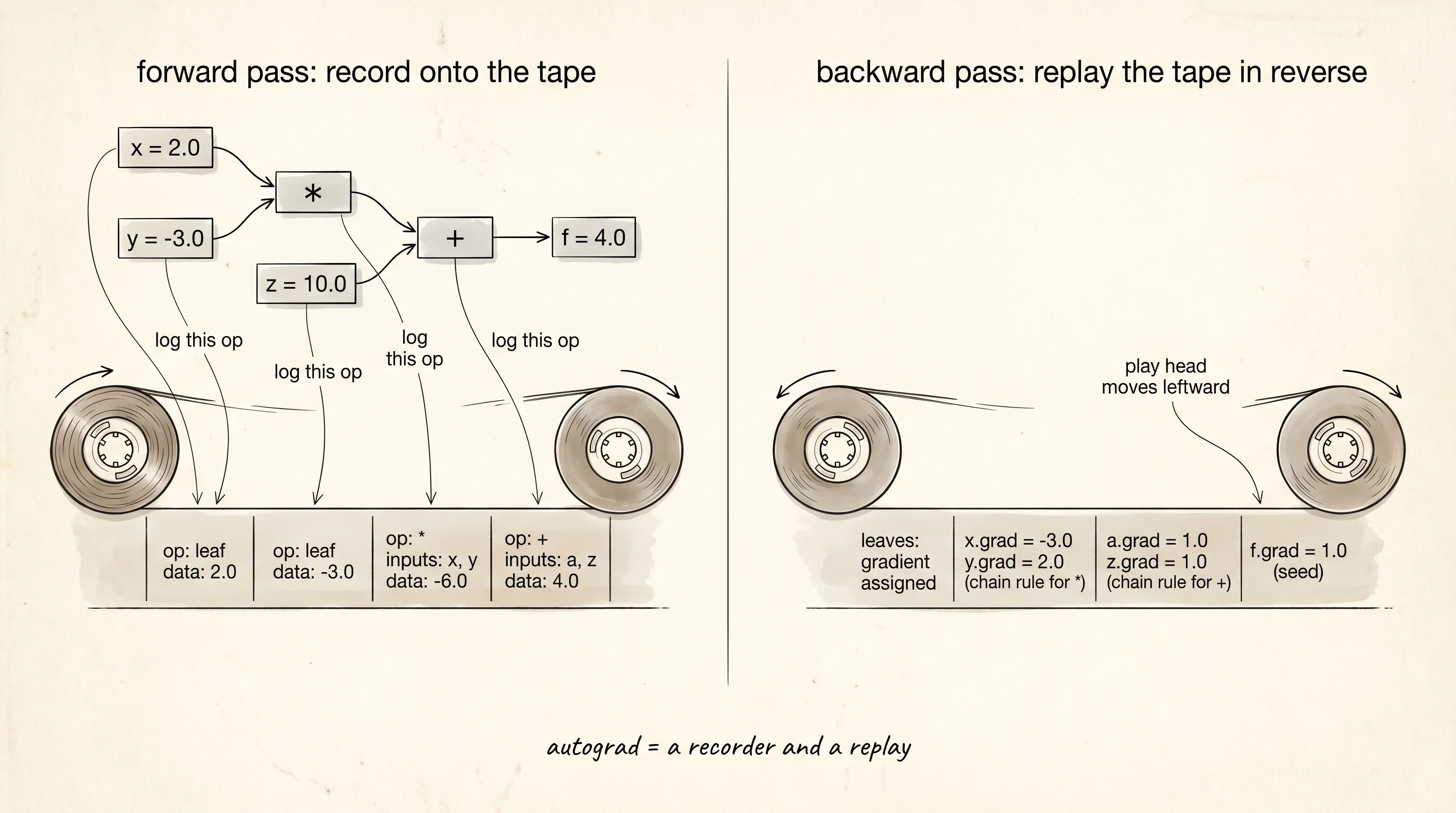
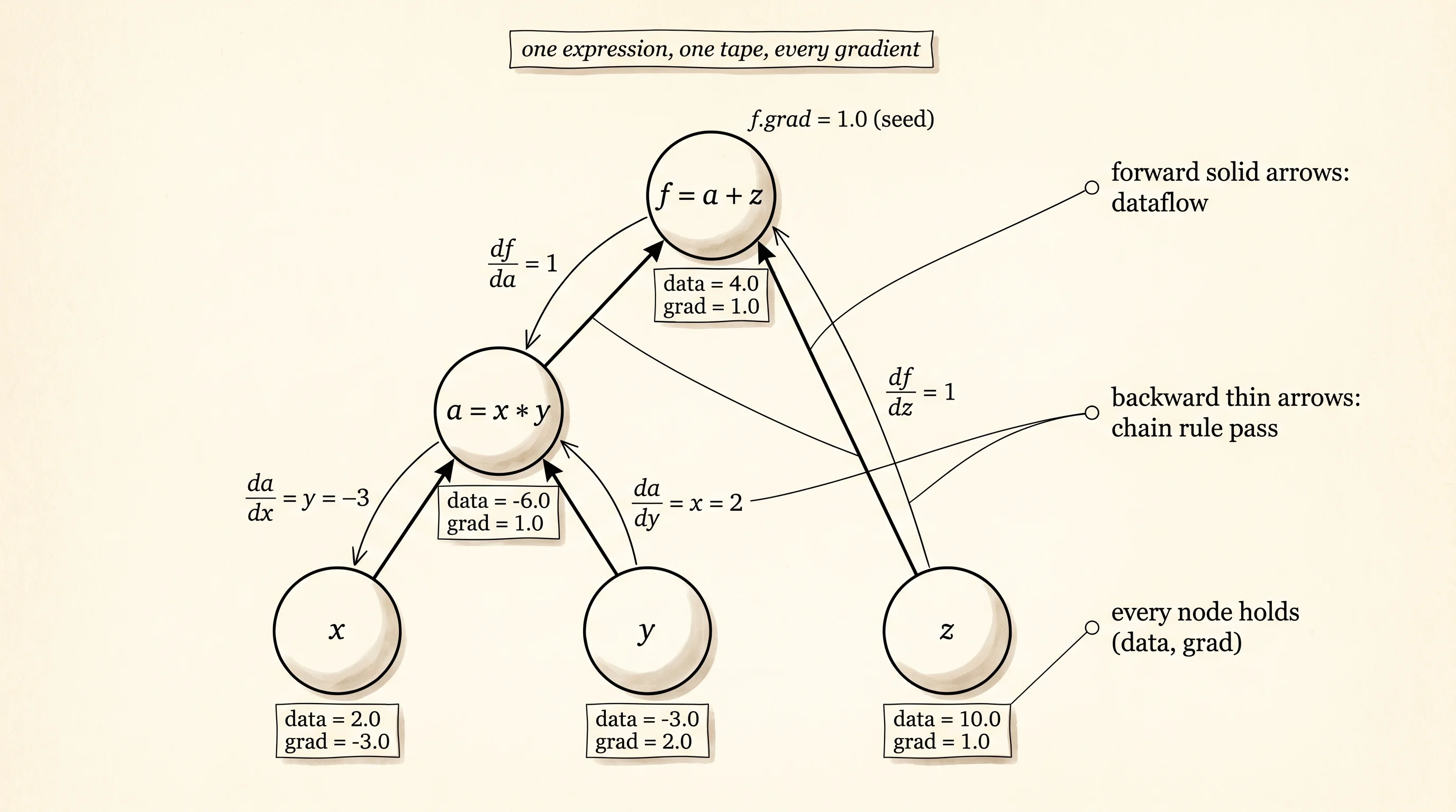
The smallest example you can hold in your head is f(x, y, z) = x * y + z. Three inputs, two operations. Build it, call backward, and print every Value in the graph.

x = Value(2.0)
y = Value(-3.0)
z = Value(10.0)
a = x * y      # a = -6
f = a + z      # f = 4
f.backward()
 
for label, node in [("x", x), ("y", y), ("z", z), ("a", a), ("f", f)]:
    print(f"{label}: {node}")

Run it.

x: Value(data=2.0000, grad=-3.0000)
y: Value(data=-3.0000, grad=2.0000)
z: Value(data=10.0000, grad=1.0000)
a: Value(data=-6.0000, grad=1.0000)
f: Value(data=4.0000, grad=1.0000)

The chain rule is sitting on the screen. df/dx = y = -3. df/dy = x = 2. df/dz = 1. df/da = 1 because f = a + z. df/df = 1 by definition. Five gradients, all correct, no derivative work. The closure attached to * knew to swap x and y for the multiplication. The closure attached to + knew to copy the upstream gradient straight through. The topological sort made sure _backward for + ran before _backward for *, so by the time the multiply step asked for a.grad, the addition step had already filled it in.

Trust comes from verification. The way to prove autograd is correct is to compare its answer against finite differences. Pick any input, nudge it by a tiny h, recompute the output, and divide the change by h. That ratio is the slope at that point. If autograd's gradient and the finite-difference slope agree to 6 or 7 decimal places across every test case, the engine is right.

def verify_gradient(f, inputs, h=1e-7):
    output = f(*inputs)
    output.backward()
    analytical = [v.grad for v in inputs]
 
    numerical = []
    for index in range(len(inputs)):
        bumped = [Value(v.data) for v in inputs]
        bumped[index].data += h
        plus = f(*bumped).data
        bumped[index].data -= 2 * h
        minus = f(*bumped).data
        numerical.append((plus - minus) / (2 * h))
 
    return analytical, numerical

Two-sided differences give a tighter answer than a single-sided bump. Run it on a few expressions a calculus student would recognize. A polynomial: g(x) = x**3 - 2*x + 5. A composition: h(x, y) = (x*y + x.exp()).tanh(). A miniature neural network: take two inputs, run them through two neurons with tanh activation, sum the outputs, square the result against a target.

def polynomial(x):
    return x ** 3 - 2 * x + Value(5.0)
 
def composed(x, y):
    return (x * y + x.exp()).tanh()
 
def tiny_network(x1, x2):
    w11, w12, w21, w22 = Value(0.5), Value(-0.3), Value(0.8), Value(0.1)
    b1, b2 = Value(0.0), Value(0.2)
    h1 = (w11 * x1 + w12 * x2 + b1).tanh()
    h2 = (w21 * x1 + w22 * x2 + b2).tanh()
    out = h1 + h2
    target = Value(1.0)
    return (out - target) ** 2
 
for name, f, inputs in [
    ("polynomial", polynomial, [Value(2.5)]),
    ("composed",   composed,   [Value(0.7), Value(-0.4)]),
    ("network",    tiny_network, [Value(1.0), Value(0.5)]),
]:
    analytical, numerical = verify_gradient(f, inputs)
    print(f"{name}:")
    for i, (a, n) in enumerate(zip(analytical, numerical)):
        print(f"  input {i}: autograd={a:+.6f}  finite_diff={n:+.6f}")

Every line agrees to 6 decimal places. The gradients come out automatically — write the forward pass once, get the backward pass for free. PyTorch is this same code with a thousand more operations and a tensor type. The flight recorder is the whole trick.

Autograd hides the chain rule behind a _backward closure on every node — once, just once, run the chain rule by hand on a tiny network so you know the engine isn't magic.