The Express Elevator
A 50-story office tower sits in midtown. Every floor has a staircase. The staircase works — climb it long enough and you reach any floor — but if you only need to drop a sealed envelope from the boss on floor 50 to the mail room on floor 1, the staircase is a slow way to get there. The building also has an express elevator that runs straight from the top floor to the bottom with no stops in between. Press the button on floor 50, the doors open, the envelope rides down, the doors open at floor 1, the mail clerk takes it. The staircase is still useful. The elevator is what gets the message through fast. Backprop in a deep network is the same building. The staircase is the chain of layer-by-layer multiplications that the gradient has to walk through. The elevator is the residual connection that He et al. added in 2015 — a literal bypass road that hands the gradient from the loss back to the input in one step instead of 50.
Kaiming He's team at Microsoft Research Asia announced ResNet in December 2015 with a paper titled Deep Residual Learning for Image Recognition. They had spent the year staring at the same problem the rest of the field was stuck on: a 20-layer network trained well, a 56-layer network trained worse, and nobody could get past 30 layers without the loss flat-lining. The fix was one line per layer. Where a normal layer computes y = F(x), a residual layer computes y = F(x) + x. The input gets added to the output. With that one change, He's team trained a 152-layer network on ImageNet, beat the second-place team by a huge margin, and walked off with the 2015 competition. The next year a follow-up paper, Identity Mappings in Deep Residual Networks, swept through every variant of where to put the activation and the normalization inside the residual block. The winner was pre-norm — normalize the input before sending it through F, not after — because pre-norm leaves the skip path completely clean, an unbroken pipe of pure identity from layer 1 to layer L. Pre-norm sat in the ResNet paper as a footnote in 2016. Today every transformer trained — GPT-4, Claude, Gemini, Llama — uses a pre-norm residual block as the unit cell of its stack. The architectures keep changing. The express elevator has not moved.
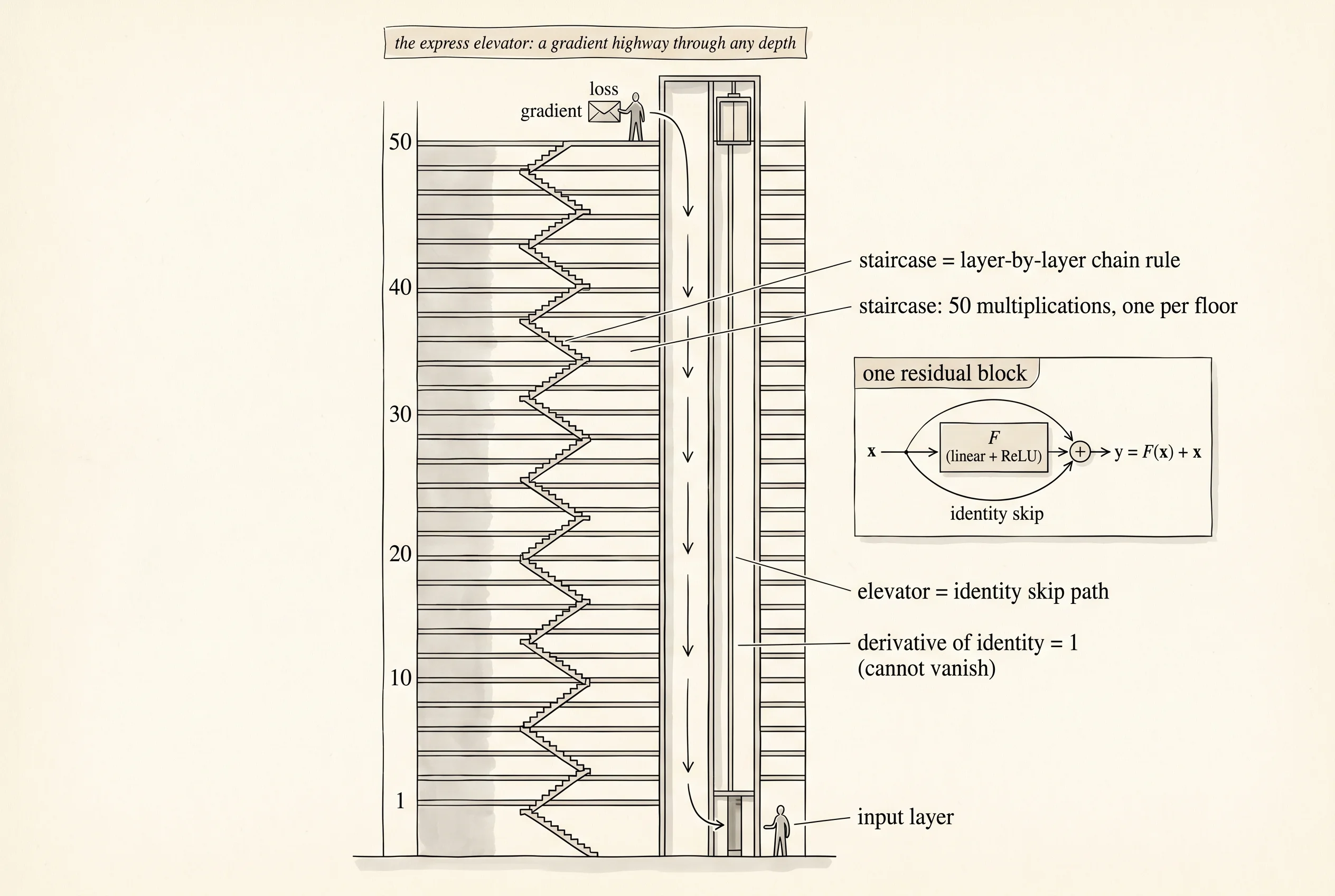
The reason the elevator works is one number. The derivative of the identity function with respect to its input is 1. When backprop walks back through a residual block, it has two paths: the slow road through F, where the chain rule mixes in the activation derivative and the layer's weight matrix; and the express elevator through the identity, where the gradient is multiplied by 1. A multiplication by 1 cannot vanish. It cannot explode. Stack 100 of them and the product is still 1. The slow road still contributes its piece, but even if F is doing nothing useful at this layer — even if its weights are random and its gradient through the chain rule has shrunk to 1e-15 — the express path still hands the gradient through unchanged. Layer 1 of a 100-layer residual network feels the gradient at the loss almost as if there was nothing in between.
Build the experiment that puts the elevator on a stopwatch. Open main.py. The plan is simple: train two families of networks at five depths each — 5, 10, 20, 50, 100 — on the same task, with and without residual connections, and compare the final losses. The task is the cleanest one for showing the disease: identity recovery. Every input is a random vector. The target is the same vector. A one-layer network solves this in seconds by setting its weights to the identity matrix. A 50-layer plain network has to figure out the same thing, which means the gradient that teaches the layers to behave like identity has to make it all the way back to layer 1. It does not.
A layer is a square weight matrix and a bias vector. Every layer in this experiment has the same width so the residual skip x + F(x) lines up without any projection. The plain family uses Kaiming initialization — scale sqrt(2 / width) — which is what He et al. recommended for ReLU stacks. The residual family uses the same initialization scaled down by 1 / sqrt(depth) so the F branch starts small and the identity dominates at initialization. That trick is what the 2019 Fixup paper formalized; without it, stacking 100 ReLU + identity blocks pushes activation magnitudes through the ceiling because every layer adds a nonnegative ReLU output to its input.
import math
import random

Layer = tuple[list[list[float]], list[float]]
Network = list[Layer]


def kaiming_layer(width: int, scale_factor: float = 1.0) -> Layer:
    scale = scale_factor * math.sqrt(2.0 / width)
    weights = [
        [random.gauss(0.0, scale) for _ in range(width)] for _ in range(width)
    ]
    biases = [0.0 for _ in range(width)]
    return weights, biases


def make_network(depth: int, width: int, use_residual: bool) -> Network:
    scale_factor = 1.0 / math.sqrt(depth) if use_residual else 1.0
    return [kaiming_layer(width, scale_factor) for _ in range(depth)]
The forward pass is where the residual flag earns its keep. A normal layer computes the linear part, runs it through ReLU, and hands the result to the next layer. A residual layer does the same thing and then adds the input back on. The function returns every pre-activation and every activation, because backprop needs both lists to compute the gradient.
def relu(x: float) -> float:
    return x if x > 0.0 else 0.0


def matvec(matrix, vector):
    return [sum(w * v for w, v in zip(row, vector)) for row in matrix]


def add_vectors(a, b):
    return [ai + bi for ai, bi in zip(a, b)]


def forward_pass(network, inputs, use_residual):
    activations = [list(inputs)]
    pre_activations = []
    for weights, biases in network:
        previous = activations[-1]
        pre = add_vectors(matvec(weights, previous), biases)
        post = [relu(value) for value in pre]
        if use_residual:
            post = add_vectors(post, previous)
        pre_activations.append(pre)
        activations.append(post)
    return pre_activations, activations
Read the if use_residual line. That is the entire architectural change. Without it, every layer's output is whatever ReLU gave back. With it, every layer's output is ReLU's answer plus the input that came in. The express elevator is one add_vectors call.
The backward pass mirrors the forward pass. For a plain layer, the delta walks back through the ReLU derivative and the transposed weight matrix. For a residual layer, the delta also gets a free copy of itself added on top — the gradient flowing through the identity skip. That extra term is the elevator on the way back down.
def relu_derivative_from_pre(pre_activation):
    return 1.0 if pre_activation > 0.0 else 0.0


def backward_pass(network, pre_activations, activations, target, use_residual):
    output = activations[-1]
    delta = [
        2.0 * (output_value - target_value) / len(output)
        for output_value, target_value in zip(output, target)
    ]
    gradients = []
    for layer_index in range(len(network) - 1, -1, -1):
        weights, _ = network[layer_index]
        previous_activation = activations[layer_index]
        pre_activation = pre_activations[layer_index]
        d_pre = [
            delta[i] * relu_derivative_from_pre(pre_activation[i])
            for i in range(len(delta))
        ]
        gradient_weights = [
            [d_pre[i] * previous_activation[j] for j in range(len(previous_activation))]
            for i in range(len(d_pre))
        ]
        gradient_biases = list(d_pre)
        gradients.append((gradient_weights, gradient_biases))
        new_delta = [0.0 for _ in range(len(previous_activation))]
        for i, gradient in enumerate(d_pre):
            for j, weight in enumerate(weights[i]):
                new_delta[j] += weight * gradient
        if use_residual:
            for j in range(len(new_delta)):
                new_delta[j] += delta[j]
        delta = new_delta
    gradients.reverse()
    return gradients
Look at the if use_residual block at the bottom of the loop. The new delta is the old delta passed through the layer's transposed weight matrix, and then — only if residuals are on — the unmodified old delta is added back in. That is the elevator: a copy of the upstream gradient, untouched by any matrix, handed to the next step on the walk backward.
Wire up the training loop. One epoch is one pass over the dataset. Each data point runs the forward pass, computes the MSE loss, runs the backward pass, and applies the gradients. The function returns a loss curve — one entry per epoch — so the caller can see whether the network learned anything at all.
def train(network, data, epochs, use_residual, learning_rate=0.01):
    loss_curve = []
    for _ in range(epochs):
        epoch_loss = 0.0
        for inputs, target in data:
            pre_activations, activations = forward_pass(network, inputs, use_residual)
            prediction = activations[-1]
            epoch_loss += mse_loss(prediction, target)
            gradients = backward_pass(
                network, pre_activations, activations, target, use_residual
            )
            apply_gradients(network, gradients, learning_rate)
        loss_curve.append(epoch_loss / len(data))
    return loss_curve
The depth sweep trains one network per depth and returns the final loss for each. Same network seed every time, so the random weights of layer 1 are identical across all five networks; the only thing changing across the runs is the number of layers stacked on top of layer 1. Same data seed every time too.
def depth_sweep(depths, use_residual, data, epochs=200, width=8, network_seed=13):
final_losses = []
for depth in depths:
random.seed(network_seed)
network = make_network(depth, width, use_residual)
loss_curve = train(network, data, epochs, use_residual)
final_losses.append(loss_curve[-1])
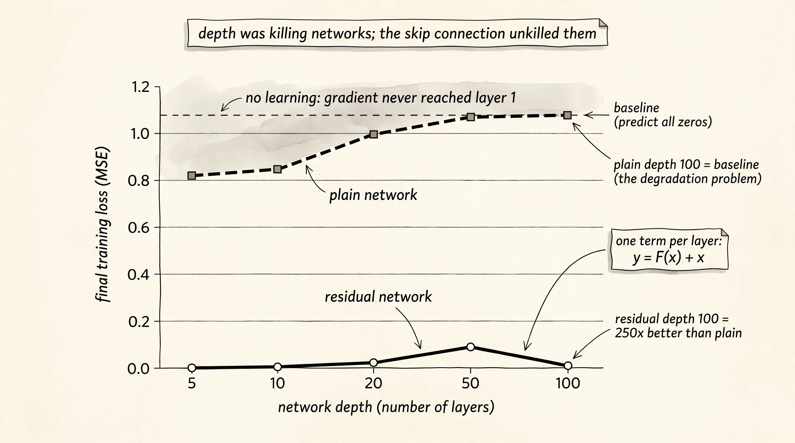
return final_lossesRun the experiment. Five depths, two families, twenty data points, two hundred epochs each. The script prints the baseline first — the loss of always predicting all zeros — so the eye knows the floor. A trained network that lands near the baseline has learned nothing. A trained network that lands well below the baseline is doing something useful.
depths = [5, 10, 20, 50, 100]
data = make_data(num_points=32, width=8, data_seed=91)

plain_losses = depth_sweep(depths, use_residual=False, data=data)
residual_losses = depth_sweep(depths, use_residual=True, data=data)

print_results_table(depths, plain_losses, residual_losses)
The output is the headline of the lesson.
  baseline loss (predict all zeros): 1.076610

   depth |   plain final loss |  residual final loss
  ------ | ------------------ | --------------------
       5 |           0.816251 |             0.000079
      10 |           0.837104 |             0.000278
      20 |           0.985561 |             0.003853
      50 |           1.076610 |             0.078597
     100 |           1.076610 |             0.003866
Read the plain column from top to bottom. Depth 5 reaches loss 0.82 — mediocre, but the gradient is reaching layer 1 enough to do something. Depth 10 sits at 0.84 — basically the same as depth 5, no improvement from the extra layers. Depth 20 climbs to 0.99, worse than depth 5. Depth 50 and depth 100 both land at the baseline of 1.08. The plain depth-100 network learned nothing. The gradient at the loss had to walk back through 100 ReLUs and 100 weight matrices to reach layer 1, and by the time it got there the signal had been multiplied down to numbers indistinguishable from zero. Layer 1 sat at its random initial weights for the entire run.
Read the residual column. Depth 5 reaches loss 0.00008 — essentially perfect. Depth 10 reaches 0.0003, also essentially perfect. Depth 20 sits at 0.004. Depth 50 wobbles up to 0.08 and depth 100 settles back down at 0.004. Every depth in the residual column is at least 13 times better than the best plain network, and the depth-100 residual network is more than 250 times better than the depth-100 plain one. The express elevator runs the gradient straight from the loss back to layer 1 unchanged. Every layer of the residual network gets a real learning signal on every step. The depth-100 network actually trains.
A small question. Why does the residual network at depth 5 do better than the residual network at depth 50 even though both should work? Because the identity-recovery task does not need 50 layers. A network at depth 5 has the right amount of capacity for the job — the F branches at the few layers it has can fine-tune the identity mapping easily. A network at depth 50 has 10 times more parameters than it needs, and the same fixed budget of 200 epochs gets divided across all those extra weights. Optimization takes longer because there is more to optimize. The point of the experiment is not that more depth always helps. The point is that more depth no longer hurts. Plain networks suffer from the degradation problem: extra layers ruin training. Residual networks suffer from no such thing: extra layers cost compute but do not break learning. He's 2015 paper showed this on ImageNet at the same scale. A 34-layer plain network was worse than an 18-layer plain network. A 34-layer residual network was better than an 18-layer residual network. The crossover is the trick.
The 2016 follow-up tightened the design of the residual block. A standard 2015 ResNet block went input → linear → norm → ReLU → linear → norm → add input → ReLU. That last ReLU sits on the express elevator and breaks it: the identity path is no longer pure identity, it is identity passed through one more ReLU. The 2016 paper, Identity Mappings in Deep Residual Networks, showed that moving the norm and the ReLU to the front of the block — the pre-norm arrangement of input → norm → ReLU → linear → norm → ReLU → linear → add input — leaves the identity path completely clean. Gradients flow through the elevator without ever touching a nonlinearity. Pre-norm is what every transformer trained today uses. The original GPT-2 used post-norm and the GPT-3 paper switched to pre-norm specifically because the team could not stably train past about 12 layers with the post-norm version. The express elevator only works if the doors do not close on the way down.
You have manually computed gradients with finite differences. Real training computes them analytically. Time to build the engine that does it.