The Gradient Telescope

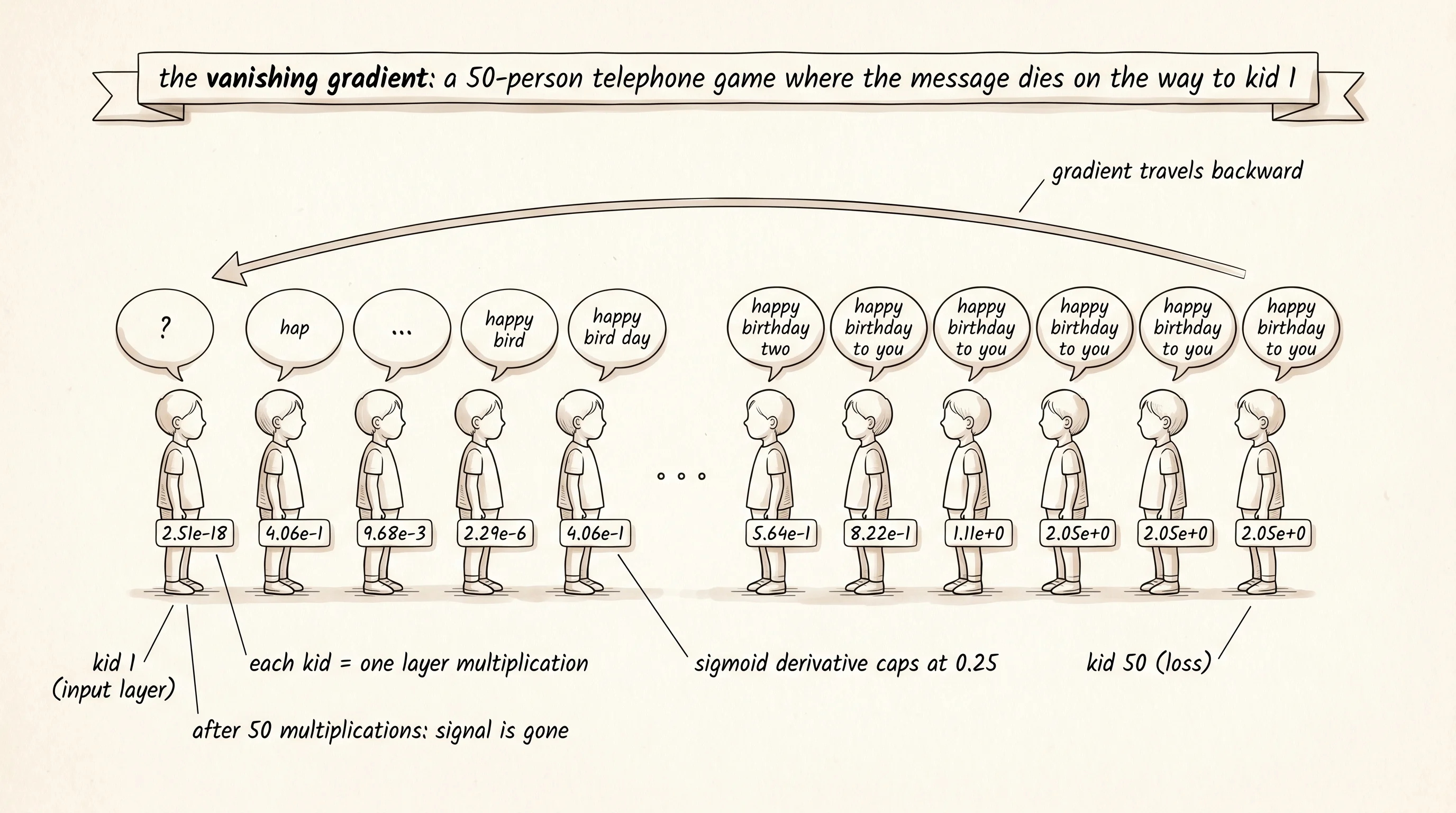
Fifty kids stand in a line for a birthday-party game. The first kid hears a sentence whispered in her ear and whispers it to the kid on her left. He whispers it to the next, and so on, all the way to the end. By the time the message reaches kid 50 it is either a complete blank — every kid trimmed off a syllable until there was nothing left — or it has been amplified into nonsense, every kid embellishing what he heard until the original sentence is buried under invented words. The original signal had to survive 50 retransmissions to make it through. It rarely does. Backprop in a deep neural network is the same line of kids. The signal is the gradient at the loss, the kids are the layers, and the message that needs to reach the first weight has to pass through 50 multiplications by 50 matrices to get there.

Sepp Hochreiter wrote this down first. In 1991, as a Diplom thesis student at TU Munich, he sat with networks of 5, 10, then 20 layers and watched the gradient at the input layer collapse to numbers so small the computer's floating-point format read them as zero. His thesis named the problem the vanishing gradient. Three years later, Yoshua Bengio, Patrice Simard, and Paolo Frasconi published the formal analysis in Learning Long-Term Dependencies with Gradient Descent is Difficult, proving that for any recurrent network trying to remember information across more than a handful of time steps, either the gradient vanishes or it explodes — and there was no setting of the weights that avoided both. Hochreiter, by then working with Jürgen Schmidhuber, gave the sequence-domain answer in 1997: the LSTM, a unit with an internal "cell" that keeps a clean copy of the past around so the gradient does not have to fight through every multiplication. The depth-domain answer waited until 2015. Kaiming He at Microsoft Research Asia trained a 152-layer ResNet on ImageNet by giving every layer a literal shortcut around itself — a bypass road for the gradient. ResNet won the competition by a record margin and the bypass road, called a residual connection, has been built into every deep network since.

The math is just multiplication. A network of depth L is L matrix multiplications stacked on top of each other. The forward pass walks left to right: the input gets multiplied by W₁, squashed by an activation, multiplied by W₂, squashed, and so on. The backward pass walks right to left: the gradient at the loss gets multiplied by the same matrices, in reverse order, with the activation derivatives mixed in. If every step shrinks the signal by a factor of 0.5, the gradient at layer 1 of a 50-layer network is the gradient at the loss times 0.5⁵⁰, which is roughly 10⁻¹⁵. Numbers that small are indistinguishable from zero. The first layer learns nothing. If every step grows the signal by a factor of 2, the gradient at layer 1 is the gradient at the loss times 2⁵⁰, which is around 10¹⁵. Numbers that large overflow and the optimizer takes a step the size of a continent. The forward pass survives both extremes — neurons saturate, or activations clip — but the backward pass does not. The whole telephone game lives or dies on the per-step factor.

Build the smallest network that shows the disease. Open gradient_telescope.py. A Network is a list of layers. A layer is a square weight matrix and a bias vector. Sigmoid is the activation. Sigmoid is a deliberate choice for this lesson — its derivative caps at 0.25, the smallest of any common activation, which is why deep sigmoid networks were the first to die.

import math
import random
 
Layer = tuple[list[list[float]], list[float]]
 
def make_layer(width: int, scale: float) -> Layer:
    weights = [
        [random.gauss(0.0, scale) for _ in range(width)] for _ in range(width)
    ]
    biases = [0.0 for _ in range(width)]
    return weights, biases
 
def make_network(depth: int, width: int, scale: float) -> list[Layer]:
    return [make_layer(width, scale) for _ in range(depth)]

The forward pass is the part that needs new behavior. A normal forward pass computes the output of each layer and returns the final one. A diagnostic forward pass saves every intermediate activation, because the backward pass needs each one to compute the gradient at that step. The function returns a list whose first entry is the input and whose last entry is the network output.

def sigmoid(x: float) -> float:
    if x < -500.0: return 0.0
    if x > 500.0:  return 1.0
    return 1.0 / (1.0 + math.exp(-x))
 
def matvec(matrix, vector):
    return [sum(w * v for w, v in zip(row, vector)) for row in matrix]
 
def add_vectors(a, b):
    return [ai + bi for ai, bi in zip(a, b)]
 
def forward_with_tracking(network, inputs, residual=False):
    activations = [list(inputs)]
    for weights, biases in network:
        previous = activations[-1]
        pre = add_vectors(matvec(weights, previous), biases)
        post = [sigmoid(value) for value in pre]
        if residual:
            post = add_vectors(post, previous)
        activations.append(post)
    return activations

The backward pass walks the saved activations in reverse and computes the gradient at every layer. The delta variable carries the gradient with respect to that layer's output as it propagates from the loss back to the input. At each step the function records the L2 norm of delta — the size of the message that layer would receive during training. That is the number the telescope reads.

def sigmoid_derivative_from_output(activation):
    return activation * (1.0 - activation)
 
def vector_l2_norm(vector):
    return math.sqrt(sum(v * v for v in vector))
 
def backward_with_tracking(network, activations, target, residual=False):
    output = activations[-1]
    delta = [o - t for o, t in zip(output, target)]
    norms = [(len(network), vector_l2_norm(delta))]
    for layer_index in range(len(network) - 1, -1, -1):
        weights, _ = network[layer_index]
        previous_activation = activations[layer_index]
        current_activation = activations[layer_index + 1]
        sig_out = (
            [current_activation[i] - previous_activation[i]
             for i in range(len(current_activation))]
            if residual else current_activation
        )
        d_pre = [delta[i] * sigmoid_derivative_from_output(sig_out[i])
                 for i in range(len(delta))]
        new_delta = [0.0] * len(previous_activation)
        for i, g in enumerate(d_pre):
            for j, w in enumerate(weights[i]):
                new_delta[j] += w * g
        if residual:
            for j in range(len(new_delta)):
                new_delta[j] += delta[j]
        delta = new_delta
        if layer_index > 0:
            norms.append((layer_index, vector_l2_norm(delta)))
    norms.reverse()
    return [norm for _, norm in norms]

Read the loop. The new delta after each step is the old delta passed through the activation derivative and then multiplied by the layer's weight matrix transposed. That multiplication is the per-step factor in the telephone game. Whether the gradient grows or shrinks depends on the typical magnitude of those matrix products composed across every layer.

A single random input draw gives a noisy reading. Average across many draws to see the typical gradient the layer would feel during training.

def average_gradient_norms(network, width, samples, residual, sample_seed):
    random.seed(sample_seed)
    accumulator = [0.0] * len(network)
    for _ in range(samples):
        inputs = [random.gauss(0.0, 1.0) for _ in range(width)]
        target = [random.gauss(0.0, 1.0) for _ in range(width)]
        activations = forward_with_tracking(network, inputs, residual=residual)
        norms = backward_with_tracking(network, activations, target, residual=residual)
        for index, value in enumerate(norms):
            accumulator[index] += value
    return [value / samples for value in accumulator]
 
def gradient_magnitude_report(depth, width, scale, residual):
    random.seed(42)
    network = make_network(depth, width, scale)
    return average_gradient_norms(network, width, samples=20,
                                  residual=residual, sample_seed=7)

Wire up the experiment. Width 4, scale 2.0 for the weights, sigmoid activation. Walk the four depths and print the gradient norm at layer 1 — the layer touching the input, the layer that has to receive the message that traveled the farthest.

for depth in [5, 10, 20, 50]:
    norms = gradient_magnitude_report(depth, width=4, scale=2.0, residual=False)
    print(f"depth {depth:2d}: layer 1 gradient norm = {norms[0]:.2e}")

Run it.

depth  5: layer 1 gradient norm = 4.06e-01
depth 10: layer 1 gradient norm = 9.68e-03
depth 20: layer 1 gradient norm = 2.29e-06
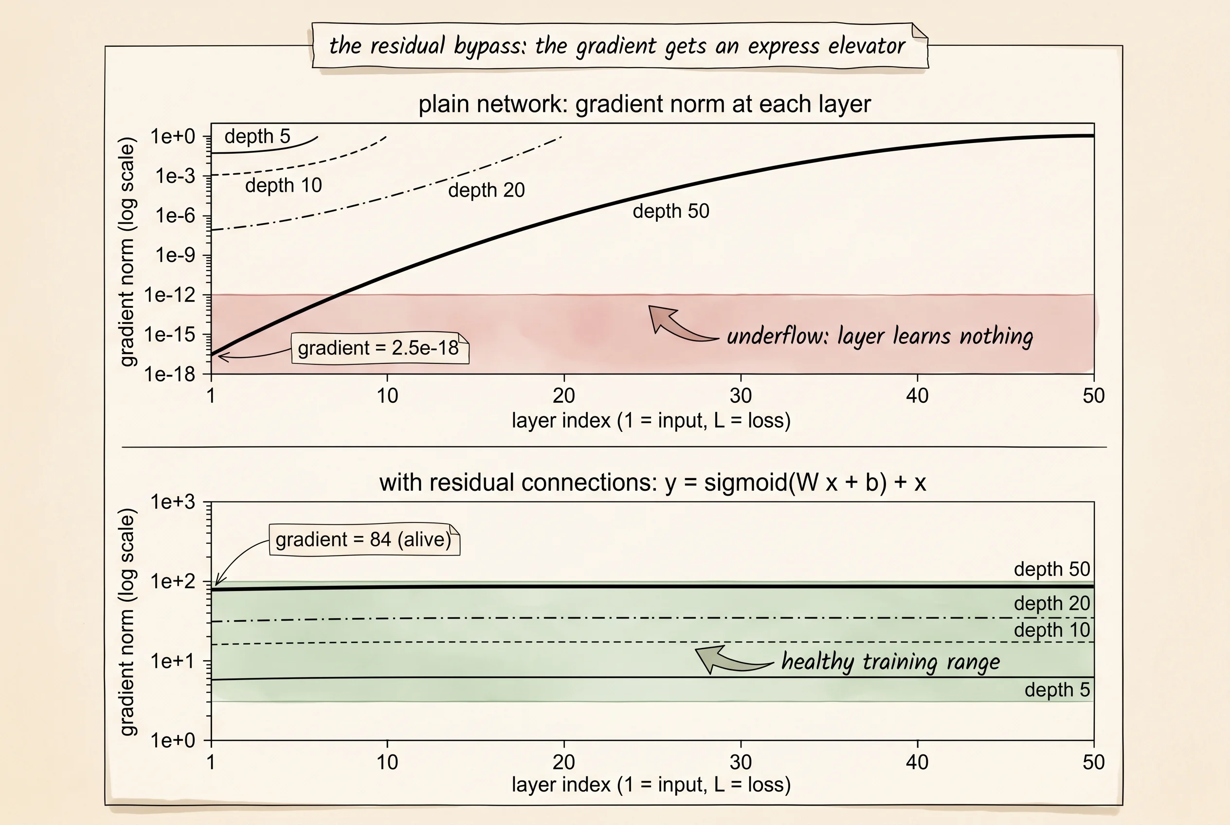
depth 50: layer 1 gradient norm = 2.51e-18

The first layer of the depth-50 network sees a gradient of 2.5 times 10 to the negative 18. That is smaller than the rounding error of a standard 32-bit float. If you tried to train this network, the optimizer would update layer 1's weights by zero on every step. Every input to the network would get processed by 50 layers of which only the last few were ever adjusted by training. The first 45 layers are frozen at their random initial values. The other side of the disease is the same shape. Push the weight scale up — try scale=4.0 and rerun — and the gradient at layer 1 starts overflowing instead of underflowing. The factor flipped from less than 1 to greater than 1. The telephone line either deletes the message or screams it.

A small question. Why does the gradient at the last layer always look healthy, no matter how deep the network is? Because the last layer is one multiplication away from the loss. The gradient there is just prediction minus target, never multiplied by anything. The deeper the network, the more layers sit between the loss and layer 1, and every one of those layers gets to fade or amplify the signal once. The first layer pays the depth tax.

Hochreiter found the disease in 1991 and the field spent two decades trying patches. Better activations — ReLU instead of sigmoid — pushed the per-step factor higher and bought maybe a factor of 4 more depth. Better initialization — Xavier and Kaiming — kept the forward pass from saturating but did not fix the backward chain. Recurrent networks, where the same matrix is multiplied by itself once per time step, were unfixable by either trick, which is why Hochreiter and Schmidhuber built the LSTM in 1997: a memory cell with an unmodified pathway through time, so the gradient could walk along the cell without being multiplied by anything. The LSTM saved sequence learning. Vision networks needed a different bypass.

Kaiming He's 2015 paper added one term to every layer. Where a normal layer computes y = F(x), a residual layer computes y = F(x) + x. The input is added to the output. The intuition is the bypass road. The math is a derivative of 1 for the skip path on top of whatever derivative F contributes — and 1 does not vanish or explode under any number of multiplications. The gradient now has two ways back to the input: the slow road through every layer's transformation, and the express elevator through the identity. The express elevator is what lets the message from layer 50 reach layer 1 still legible.

Wiring residuals into the existing code is one line each in the forward and backward pass — already in the snippets above, gated by the residual flag. Rerun the experiment with the flag on.

for depth in [5, 10, 20, 50]:
    norms = gradient_magnitude_report(depth, width=4, scale=2.0, residual=True)
    print(f"depth {depth:2d}: layer 1 gradient norm = {norms[0]:.2e}")

The output is a different world.

depth  5: layer 1 gradient norm = 6.76e+00
depth 10: layer 1 gradient norm = 1.72e+01
depth 20: layer 1 gradient norm = 3.28e+01
depth 50: layer 1 gradient norm = 8.39e+01

Layer 1 of the depth-50 network now sees a gradient of 84. Compare that to the 2.5 times 10 to the negative 18 it saw without residuals. The telephone game just got an express telephone wire from the last kid to the first. The signal at the deep end is bigger than the signal at the shallow end now — the gradient adds a fresh contribution at every layer through the skip path, and those contributions accumulate as you walk backward. The number is larger than 1, not exactly equal to 1, but the disease is gone. Every layer of the 50-layer residual network is trainable. None of them are frozen. The 152-layer ResNet that won ImageNet 2015 was the same trick built at scale. Every transformer trained today — GPT-4, Claude, Gemini — has a residual connection around every single attention block and every single feedforward block in the stack. The architectures keep changing. The bypass road has not moved.

Residual connections fixed it for you. Now build them yourself and see why.