Weight Initialization

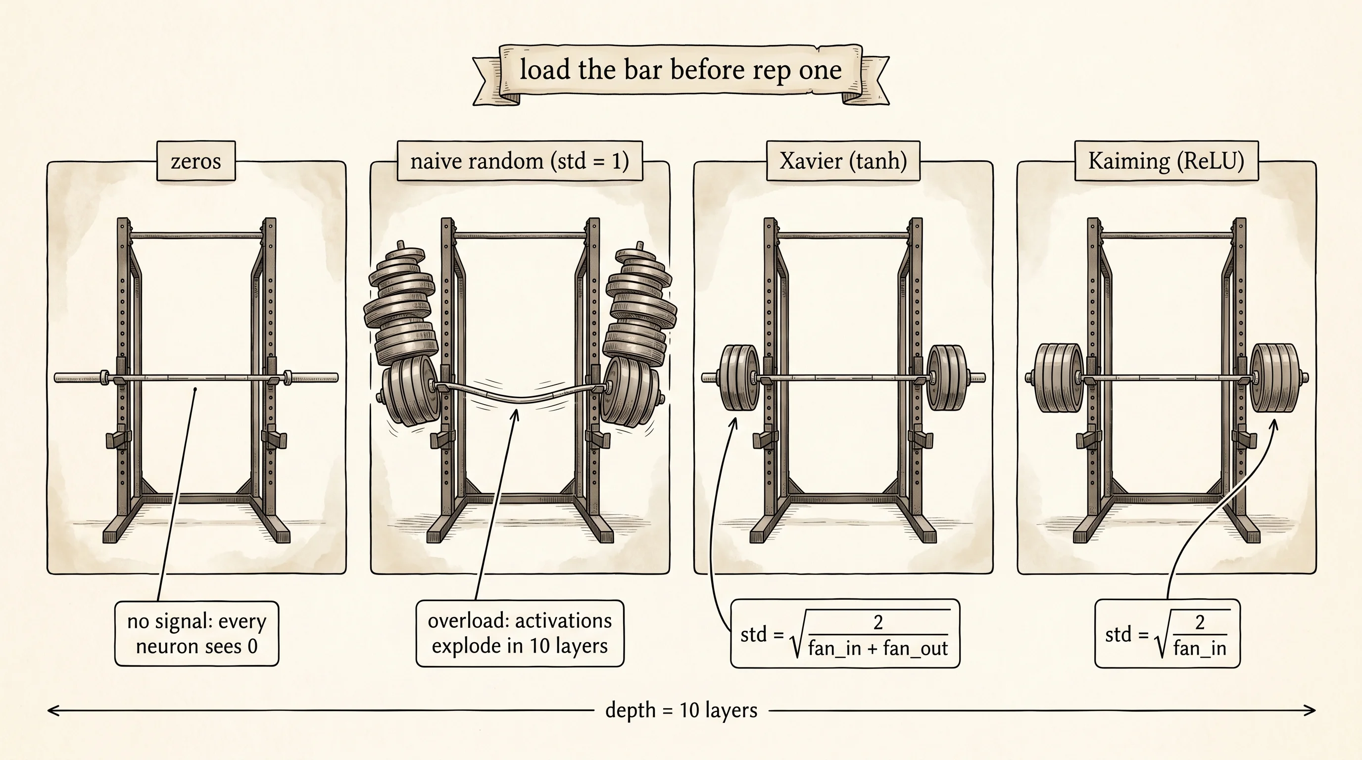
The optimizer needs a gradient. The gradient needs the loss. The loss needs a forward pass. And the forward pass needs weights — numbers that exist before the first batch is ever seen. Loading the bar before the first set is the same problem. Empty bar and you cannot tell what you are lifting; nothing moves and nothing teaches you anything. Pile on 405 pounds and your back goes out before rep one. The right plates calibrated to your actual strength let you start the workout. Pick the wrong starting weights for a network and the same two failures show up: every activation pinned to zero, or every activation rocketing into the millions before the first layer finishes.

For most of neural-network history nobody noticed this was a problem. People used random small numbers and trained shallow networks where it almost did not matter. In 2010 Xavier Glorot and Yoshua Bengio at the Université de Montréal wrote Understanding the difficulty of training deep feedforward neural networks. They asked one question: as you stack more layers, why does training get harder? The paper traced the answer to the variance of the activations. If each layer multiplies the input by a weight matrix and the weights are too big, the variance grows by a factor every layer; ten layers of 2x growth and your activations are 1024 times the input. Too small and the variance shrinks to nothing. Glorot and Bengio derived the right scale — variance equals 2 divided by (fanin plus fan_out) — to keep activations near unit scale through arbitrary depth, assuming the activation function is tanh or linear. Five years later Kaiming He and his coauthors at Microsoft Research published _Delving Deep into Rectifiers. The Glorot derivation assumed a symmetric activation. ReLU is not symmetric — it sets half its inputs to zero, which cuts the variance in half on every layer. He's fix was a single edit: double the variance to 2 divided by fan_in. That one line let them train a 152-layer ResNet that won ImageNet 2015 by a wide margin. In 2021 Greg Yang and Edward Hu's μP paper extended init theory further, showing that the right scaling law also lets hyperparameters transfer across model sizes — the learning rate that worked at 100 million parameters keeps working at 100 billion parameters if the init is right.

A network is a stack of layers, each one a matrix multiply followed by a nonlinearity. Build a 10-layer version where every layer is square — 64 inputs into 64 outputs — and forget about biases for now. Strip off the activation function for one second and look at a single layer. The activation at neuron i in the next layer is the dot product of 64 weights and 64 inputs. If the inputs have variance 1 and the weights have variance v, the output has variance 64 times v. Run that math through ten layers and the variance after layer 10 is 64^10 * v^10 times the input variance. With v = 1 the activation variance is around 10^18. With v = 0.001 it is around 10^-30. There is exactly one choice of v that keeps the variance constant across layers — v = 1 / 64, which is 1 / fan_in. That single observation is the entire content of every initialization scheme; the rest is bookkeeping for the activation function in between.

import math
import random
 
 
def init_zeros(fan_in, fan_out):
    return [[0.0 for _ in range(fan_in)] for _ in range(fan_out)]
 
 
def init_random(fan_in, fan_out):
    return [
        [random.gauss(0.0, 1.0) for _ in range(fan_in)]
        for _ in range(fan_out)
    ]
 
 
def init_xavier(fan_in, fan_out):
    std = math.sqrt(2.0 / (fan_in + fan_out))
    return [
        [random.gauss(0.0, std) for _ in range(fan_in)]
        for _ in range(fan_out)
    ]
 
 
def init_kaiming(fan_in, fan_out):
    std = math.sqrt(2.0 / fan_in)
    return [
        [random.gauss(0.0, std) for _ in range(fan_in)]
        for _ in range(fan_out)
    ]

Four functions and they fit on one screen. init_zeros returns a matrix of zeros. init_random draws every weight from a unit Gaussian — no scaling at all, the naive thing a beginner reaches for. init_xavier uses Glorot's formula. init_kaiming uses He's formula. The only thing that changes between them is the standard deviation of the Gaussian. None of them needs a single line of math more than what is on the screen.

Wire them into a 10-layer network and add the two activation functions you have already met: tanh, which squashes any number into the range (-1, 1), and relu, which zeros out negatives and passes positives through.

class Network:
    def __init__(self, num_layers, layer_width, initializer, activation):
        self.activation = activation
        self.weights = [
            initializer(layer_width, layer_width) for _ in range(num_layers)
        ]
 
 
def matmul_vector(matrix, vector):
    out = []
    for row in matrix:
        total = 0.0
        for weight, value in zip(row, vector):
            total += weight * value
        out.append(total)
    return out
 
 
def forward_with_stats(network, input_vector):
    stats = []
    activations = input_vector
    for weight_matrix in network.weights:
        pre_activations = matmul_vector(weight_matrix, activations)
        activations = [network.activation(value) for value in pre_activations]
        mean = sum(activations) / len(activations)
        variance = sum((v - mean) ** 2 for v in activations) / len(activations)
        stats.append((mean, math.sqrt(variance)))
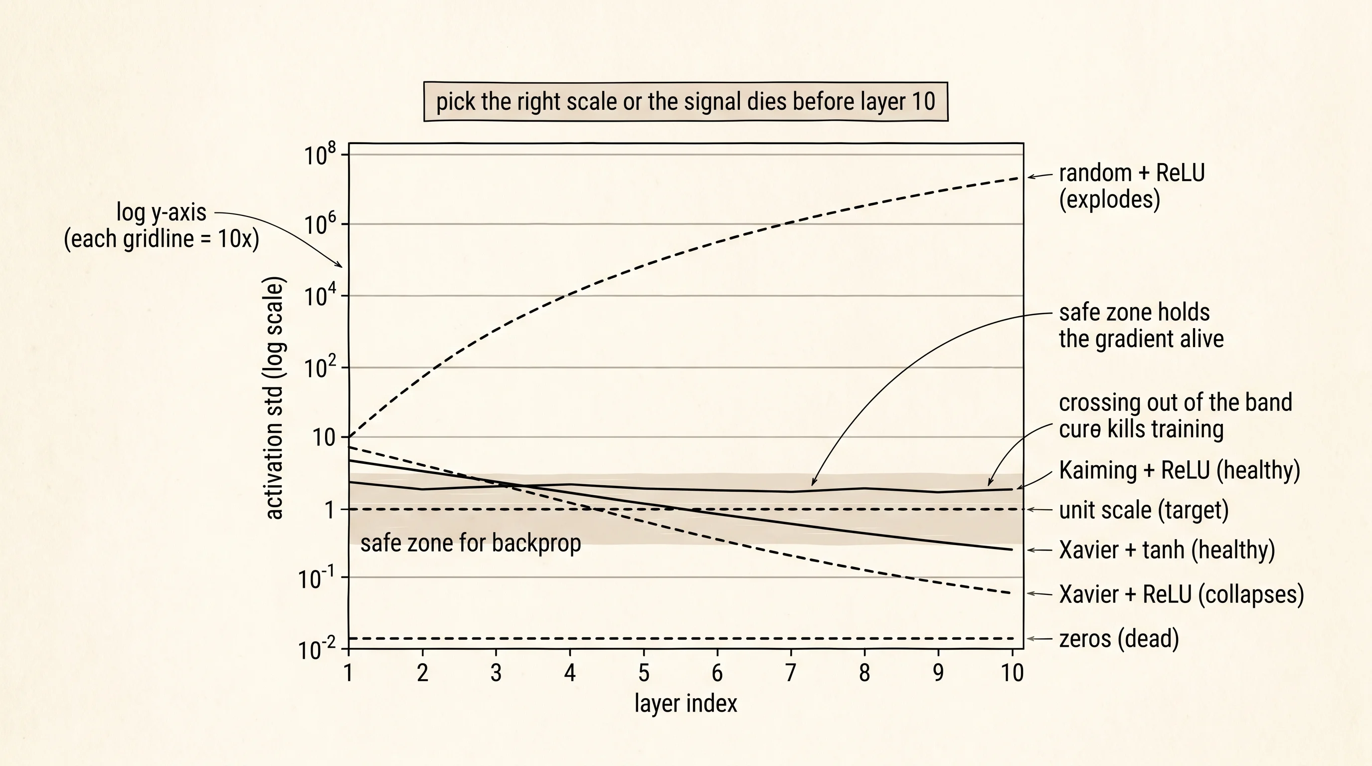
    return stats

forward_with_stats does one job: walk the layers, multiply, apply the activation, then record the mean and standard deviation of every activation vector. The standard deviation is the number that matters. If it stays near 1 from layer 1 through layer 10, the network is healthy. If it collapses to zero, every neuron is dead and there is no signal left to teach. If it explodes into the millions, the next layer's inputs are saturating every nonlinearity and the gradient through them is also dead.

Run all four initializers paired with tanh, then all four paired with ReLU. Eight runs total. Use the same random input vector for every run so the only thing changing is the weight matrix.

random.seed(7)
input_vector = [random.gauss(0.0, 1.0) for _ in range(64)]
 
initializers = [("zeros", init_zeros), ("random", init_random),
                ("xavier", init_xavier), ("kaiming", init_kaiming)]
activations = [("tanh", math.tanh), ("relu", lambda x: x if x > 0.0 else 0.0)]
 
for activation_name, activation in activations:
    for init_name, initializer in initializers:
        random.seed(7)
        network = Network(10, 64, initializer, activation)
        stats = forward_with_stats(network, input_vector)
        final_std = stats[-1][1]
        print(f"{init_name:>8s} + {activation_name:<5s}  layer-10 std = {final_std:.3e}")

The output is the punchline of the entire lesson. Read the std at layer 10 for each combination.

   zeros + tanh   layer-10 std = 0.000e+00
  random + tanh   layer-10 std = 9.224e-01
  xavier + tanh   layer-10 std = 1.980e-01
 kaiming + tanh   layer-10 std = 4.983e-01
   zeros + relu   layer-10 std = 0.000e+00
  random + relu   layer-10 std = 5.255e+07
  xavier + relu   layer-10 std = 4.894e-02
 kaiming + relu   layer-10 std = 1.566e+00

Zeros is dead in both columns. Every weight is zero, so every pre-activation is zero, so every activation is zero, so layer 10 is full of zeros. The forward pass produces no signal. Backprop will produce no gradient. The network has the same expressive power as a single neuron and zero training will ever change that fact, because every neuron in every layer sees the same input and produces the same output and computes the same gradient. Symmetry is unbreakable when you start from zero.

Random with ReLU is the explosion the curriculum promised. The standard deviation at layer 10 is 5.3 times 10 to the seventh — 53 million. Each layer's pre-activations have variance 64 times the input variance. ReLU passes the positives through unchanged. Stacking ten of them multiplies the variance by roughly (64 / 2)^10, which is around 10^15. After taking the square root for the standard deviation, you get exactly the 10^7 the table shows. Any reasonable loss function on activations of size 50 million is going to compute a gradient of size 50 million squared, and the first weight update will fling every parameter into a number too big for floating point to hold.

Random with tanh looks like it survived — std around 0.92. It did not. Tanh saturates: inputs much bigger than 3 in absolute value get squashed to almost exactly +1 or -1. The activations are bounded by definition, so the std cannot go above 1. What is hidden by the std is that almost every neuron is sitting at the flat part of the tanh curve where the derivative is essentially zero. Forward pass alive; backward pass dead. The std lied. This is exactly why initialization research had to include a backward-pass argument, not just a forward-pass argument.

Xavier with tanh holds the std at 0.198 at layer 10 — small but stable, no collapse, no explosion, and the activations sit in the linear region of tanh where the derivative is large. Kaiming with ReLU is the cleanest of the eight: std equals 1.566 at layer 10, almost exactly unit scale, exactly the property both papers were derived to give. The two cross-pairings — Xavier with ReLU and Kaiming with tanh — drift but do not blow up. Xavier with ReLU collapses (0.049) because ReLU eats half the variance every layer and Xavier never compensated. Kaiming with tanh stays around 0.5 because Kaiming overshoots tanh's already-bounded output by a factor of 2.

A small question. If Kaiming is just Xavier with twice the variance, why does Kaiming outperform Xavier on ReLU? Because ReLU drops every input below zero. A weight matrix with mean-zero rows lights up half its outputs and zeros the other half on average. The variance of the surviving half is exactly half of what the matrix would produce on a symmetric activation. Doubling the input variance — which is what 2/fan_in does compared to 2/(fan_in + fan_out) — exactly cancels the halving. The factor of 2 in Kaiming's formula is the exact accounting fee ReLU charges for setting half of its inputs to zero.

The same line of reasoning is why Xavier's denominator has fan*in plus fan_out and not just fan_in. The forward pass cares about fan_in: the variance of the output depends on how many inputs each output sums over. The backward pass cares about fan_out: the gradient at each weight depends on how many outputs the same input feeds into. Xavier picked the average of the two so that the activation variance and the gradient variance both stay near 1 as you walk forward and back through the network. Kaiming dropped the fan_out because in their experiments the forward-pass argument turned out to dominate; later work has alternated between using fan_in and fan_avg depending on the layer. Every variant traces back to the same scaling derivation, and every modern framework — PyTorch's nn.init.kaiming_normal*, JAX's initializers, every transformer trained today — uses one of these formulas as its default.

The point of the print moment is not the precise std numbers. The point is that 4 of the 8 combinations are immediately catastrophic before any training has happened. Zero gradient information leaves layer 10 in 4 of the 8 setups. The other 4 carry signal through. The choice of initialization is a pre-condition for training; it is not a hyperparameter you tune later. Pick wrong and the network never learns; pick right and the optimizer from the previous lesson finally has a gradient worth descending.

Bad init kills the forward pass — and even with good init, a different death waits for the backward pass in deep networks.