The Optimizer Race
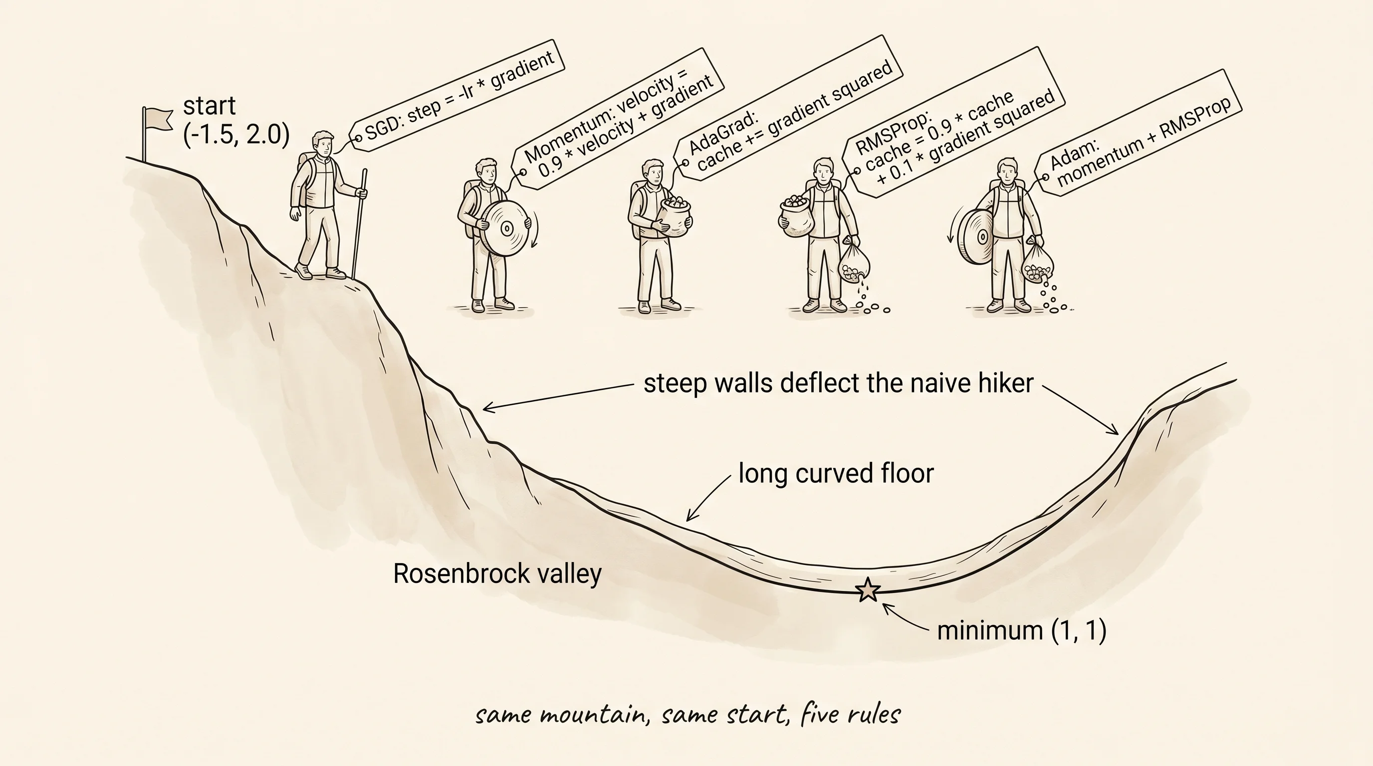
Five hikers stand at the same spot near the top of a mountain. The mountain is the loss surface, the bottom of the valley is the answer, and every hiker is trying to reach it first. The first hiker walks straight downhill, every step the same length, no memory of the last one. The second hiker keeps a running tally of which way she has been moving and lets that tally carry her forward when the slope agrees. The third hiker starts fast and keeps a list of how much each foot has been working — the foot that has done a lot of work gets shorter and shorter steps. The fourth hiker does the same but only remembers the last few steps. The fifth hiker is doing both at once. They are vanilla SGD, momentum, AdaGrad, RMSProp, and Adam, and they are about to race down the same Rosenbrock valley.
Boris Polyak put the first one on the map in 1964. He was a Soviet mathematician working on optimization theory in Moscow, and the problem he kept hitting was that ordinary gradient descent zig-zags across narrow ravines instead of running down them. His fix in a short Russian-language paper was to add a velocity term — the next step copies a fraction of the previous step, scaled by a momentum coefficient. The math was three lines. Nobody outside the Soviet optimization community paid attention for thirty years. When neural network training took off in the 1990s, people kept rediscovering the same trick under different names — heavy ball, Nesterov momentum, classical momentum — and Polyak's paper finally got the citations. John Duchi, Elad Hazan, and Yoram Singer were the next move, in 2011 at Berkeley and Google. Their paper introduced AdaGrad, the first optimizer that gave every parameter its own learning rate, scaled down by how much that parameter had been updated in the past. AdaGrad was great for sparse data — a word that appears in 1 of every 10000 documents was no longer drowned out by a word that appeared in every document. The problem was the cache only grew, so eventually every step shrank to almost nothing and training froze. One year later in a 2012 Coursera lecture, Geoffrey Hinton and his student Tijmen Tieleman showed a one-line fix: replace the growing cache with an exponential moving average. They called it RMSProp. There was never a paper. The slide in Hinton's lecture became one of the most cited "papers" in deep learning history, even though there was no paper to cite. In 2015 Diederik Kingma and Jimmy Ba in Toronto wrote down what was already obvious to anyone who had used both Polyak's momentum and Hinton's RMSProp in the same week: do both at once. They called it Adam, short for adaptive moment estimation. The paper became the most-cited optimizer paper in the history of the field and the default optimizer in every deep learning library. Ilya Loshchilov and Frank Hutter at Freiburg published one more correction in 2019: Adam handled weight decay wrong, and decoupling it gave a noticeably better optimizer they called AdamW. Every modern training script reaches for AdamW first.
The previous lesson left you with one optimizer that zig-zags down narrow ravines and crawls across plateaus. The fix every other optimizer on this page builds on is a buffer that remembers where the hiker has been. Vanilla SGD has no memory. Every step starts fresh. The update rule is one line: subtract the learning rate times the gradient from the current position.
class SGD:
    def __init__(self, x, y, learning_rate=0.001):
        self.x = x
        self.y = y
        self.learning_rate = learning_rate

    def step(self, gradient):
        dx, dy = gradient
        self.x -= self.learning_rate * dx
        self.y -= self.learning_rate * dy
        return self.x, self.y
Read it twice. Subtract gradient times learning rate from each coordinate. Return the new position. That is gradient descent in 4 lines of method body, and the rest of the page is about what to add to fix what this version cannot do.
Momentum adds one extra number per parameter, called velocity. The velocity at step t is the velocity at step t-1, scaled by a momentum coefficient (almost always 0.9), plus the current gradient. The actual position update uses the velocity, not the raw gradient. A consistent slope builds the velocity up over many steps; a jittery slope cancels itself out in the running sum.
class MomentumSGD:
    def __init__(self, x, y, learning_rate=0.001, momentum=0.9):
        self.x = x
        self.y = y
        self.learning_rate = learning_rate
        self.momentum = momentum
        self.vx = 0.0
        self.vy = 0.0

    def step(self, gradient):
        dx, dy = gradient
        self.vx = self.momentum * self.vx + dx
        self.vy = self.momentum * self.vy + dy
        self.x -= self.learning_rate * self.vx
        self.y -= self.learning_rate * self.vy
        return self.x, self.y
The velocity is an exponential moving average. With momentum at 0.9, the gradient from 10 steps ago still contributes about a third of its original weight to the current velocity. The hiker is not deciding where to go from where she is. She is deciding where to go from where she has been heading.
AdaGrad takes a different angle. Instead of remembering direction, it remembers magnitude. Every parameter keeps a running sum of squared past gradients. Each step divides the gradient by the square root of that sum, plus a tiny epsilon so the math never divides by zero. A parameter that has been updated hard takes smaller and smaller steps. A parameter that has barely moved keeps its full step size. The result is automatic per-parameter learning rate tuning.
import math

class AdaGrad:
    def __init__(self, x, y, learning_rate=0.5, epsilon=1e-8):
        self.x = x
        self.y = y
        self.learning_rate = learning_rate
        self.epsilon = epsilon
        self.cache_x = 0.0
        self.cache_y = 0.0

    def step(self, gradient):
        dx, dy = gradient
        self.cache_x += dx * dx
        self.cache_y += dy * dy
        self.x -= self.learning_rate * dx / (math.sqrt(self.cache_x) + self.epsilon)
        self.y -= self.learning_rate * dy / (math.sqrt(self.cache_y) + self.epsilon)
        return self.x, self.y
The flaw is in the line cache_x += dx * dx. The cache only grows. After 10000 steps the denominator is enormous and every step is tiny, even if the surface still has miles of slope to descend. AdaGrad is brilliant on the first thousand steps and dead on the ten-thousandth.
RMSProp swaps the running sum for an exponential moving average — the same trick momentum used on the gradient itself, but applied to the squared gradient. The cache forgets old movement. The decay coefficient is almost always 0.9, which means the cache half-life is around 7 steps. The step size never collapses to zero.
class RMSProp:
    def __init__(self, x, y, learning_rate=0.01, decay=0.9, epsilon=1e-8):
        self.x = x
        self.y = y
        self.learning_rate = learning_rate
        self.decay = decay
        self.epsilon = epsilon
        self.cache_x = 0.0
        self.cache_y = 0.0

    def step(self, gradient):
        dx, dy = gradient
        self.cache_x = self.decay * self.cache_x + (1.0 - self.decay) * dx * dx
        self.cache_y = self.decay * self.cache_y + (1.0 - self.decay) * dy * dy
        self.x -= self.learning_rate * dx / (math.sqrt(self.cache_x) + self.epsilon)
        self.y -= self.learning_rate * dy / (math.sqrt(self.cache_y) + self.epsilon)
        return self.x, self.y
Adam is momentum and RMSProp glued together. Two running averages per parameter: the first moment is the moving average of the gradient (momentum, with beta1 around 0.9) and the second moment is the moving average of the squared gradient (RMSProp, with beta2 around 0.999). Both averages start at zero, which biases them low for the first few steps, so Adam adds a bias correction that scales each average by 1 / (1 - beta**t). The actual update is the bias-corrected first moment divided by the square root of the bias-corrected second moment.
class Adam:
    def __init__(self, x, y, learning_rate=0.05, beta1=0.9, beta2=0.999, epsilon=1e-8):
        self.x = x
        self.y = y
        self.learning_rate = learning_rate
        self.beta1 = beta1
        self.beta2 = beta2
        self.epsilon = epsilon
        self.m_x = 0.0
        self.m_y = 0.0
        self.v_x = 0.0
        self.v_y = 0.0
        self.t = 0

    def step(self, gradient):
        dx, dy = gradient
        self.t += 1
        self.m_x = self.beta1 * self.m_x + (1.0 - self.beta1) * dx
        self.m_y = self.beta1 * self.m_y + (1.0 - self.beta1) * dy
        self.v_x = self.beta2 * self.v_x + (1.0 - self.beta2) * dx * dx
        self.v_y = self.beta2 * self.v_y + (1.0 - self.beta2) * dy * dy
        m_hat_x = self.m_x / (1.0 - self.beta1 ** self.t)
        m_hat_y = self.m_y / (1.0 - self.beta1 ** self.t)
        v_hat_x = self.v_x / (1.0 - self.beta2 ** self.t)
        v_hat_y = self.v_y / (1.0 - self.beta2 ** self.t)
        self.x -= self.learning_rate * m_hat_x / (math.sqrt(v_hat_x) + self.epsilon)
        self.y -= self.learning_rate * m_hat_y / (math.sqrt(v_hat_y) + self.epsilon)
        return self.x, self.y
The five classes are the inventory. To race them, give each one the same starting point on the same surface, hand each one a noisy gradient at every step, and let them run for 400 steps. The Rosenbrock function is the standard hard-mode test bed: a long curved valley with steep walls, minimum at (1, 1). Real training never sees the true gradient — every mini-batch is a fresh random sample of the data, so the gradient jiggles around the truth. Add Gaussian noise to a finite-difference gradient to simulate that jiggle.
import random

def rosenbrock(x, y):
    return (1.0 - x) ** 2 + 100.0 * (y - x * x) ** 2

def numerical_gradient(f, x, y, h=1e-5):
    dx = (f(x + h, y) - f(x - h, y)) / (2.0 * h)
    dy = (f(x, y + h) - f(x, y - h)) / (2.0 * h)
    return dx, dy

def noisy_gradient(f, x, y, noise_std):
    dx, dy = numerical_gradient(f, x, y)
    dx += random.gauss(0.0, noise_std)
    dy += random.gauss(0.0, noise_std)
    return dx, dy

def race(optimizers, f, start, steps, noise_std=0.5):
    paths = {opt.name: [(start[0], start[1], f(*start))] for opt in optimizers}
    for _ in range(steps):
        for opt in optimizers:
            gradient = noisy_gradient(f, opt.x, opt.y, noise_std)
            new_x, new_y = opt.step(gradient)
            paths[opt.name].append((new_x, new_y, f(new_x, new_y)))
    return paths
Run it. Start every hiker at (-1.5, 2.0), 400 steps, noise standard deviation 0.5. Print the loss for every optimizer at a handful of snapshot steps.
  step |        SGD |   Momentum |    AdaGrad |    RMSProp |       Adam
-----------------------------------------------------------------------
     0 |    12.5000 |    12.5000 |    12.5000 |    12.5000 |    12.5000
     1 |    11.3096 |    11.3277 |   229.0000 |     7.6431 |     6.2781
     5 |     6.6797 |     7.6500 |     6.1169 |     5.9405 |     7.2757
    25 |     5.7928 |     5.4135 |     5.8081 |     5.8802 |     5.9134
   100 |     5.6040 |     2.4865 |     5.5159 |     5.5076 |     5.1479
   200 |     5.3491 |     0.1394 |     5.1388 |     4.9066 |     3.6391
   400 |     4.7733 |     0.0130 |     4.3563 |     3.1995 |     0.3776
Five different personalities in one table. Vanilla SGD takes 400 steps to drop the loss from 12.5 to 4.8 — it is moving, but the curved valley keeps deflecting it sideways. Momentum is the cleanest run: by step 100 it is at 2.5, by step 200 it is at 0.14, by step 400 it is at 0.01 — basically at the minimum. The accumulated velocity carries it through the curve. AdaGrad takes one giant step on iteration 1 (the first squared cache is small, so the denominator is small, so the step is big — the loss spikes to 229) then settles, but the only-growing cache strangles its later steps. RMSProp avoids the spike and keeps moving but never finds the real groove. Adam splits the difference: a controlled first jump to 6.3, then steady descent, ending at 0.38 — past most of the valley and closing in.
A small question. Why does momentum beat Adam here when Adam is supposed to be the best optimizer in deep learning? Because the Rosenbrock surface is small and the noise is tame, and Adam's per-parameter rate scaling buys you nothing on a surface where both parameters need similar scales. The features that make Adam dominate real training — millions of parameters, sparse gradients, varying scales across layers — are not present in a 2-dimensional toy. Momentum is enough when the geometry is clean. Adam wins when the geometry is messy, which is every actual neural network ever trained.
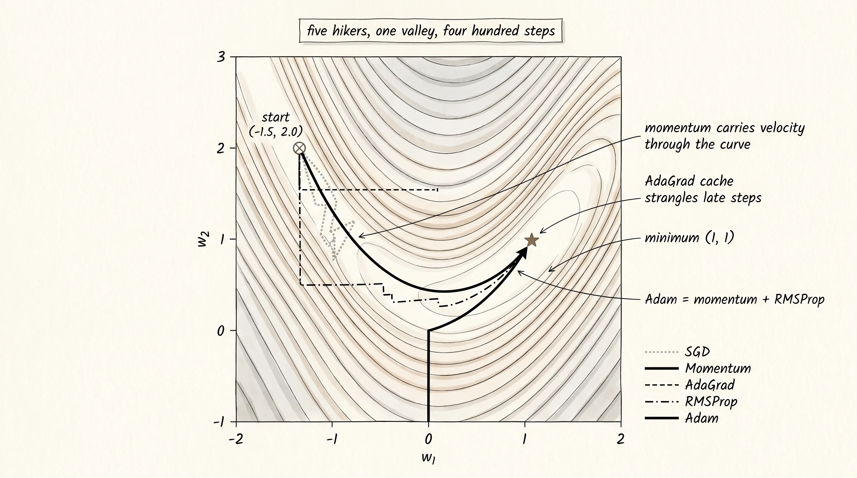
Print where every optimizer ended up after 400 steps and the same story shows up in distance from the target.
final positions vs target (1.00, 1.00):
   optimizer |   final x |   final y |  distance |  final loss
  ------------------------------------------------------------
         SGD |   -1.1825 |    1.4083 |    2.2204 |      4.7733
    Momentum |    0.8878 |    0.7862 |    0.2414 |      0.0130
     AdaGrad |   -1.0865 |    1.1858 |    2.0948 |      4.3563
     RMSProp |   -0.7873 |    0.6269 |    1.8258 |      3.1995
        Adam |    0.3858 |    0.1468 |    1.0513 |      0.3776
Momentum lands within 0.24 of the target. Adam closes the distance from 3.5 (the start) to 1.05. SGD, AdaGrad, and RMSProp barely cross the halfway mark. Momentum's accumulated velocity rides the curved valley floor; Adam's adaptive rate would have caught up given another 200 steps. The other three are fighting the geometry.
Every one of these classes has a learning rate, and the learning rates that worked here are all different. SGD wanted 0.001. AdaGrad wanted 0.5. Adam wanted 0.05. RMSProp wanted 0.01. Pick the wrong learning rate for any of them and the run looks broken. The reason Adam became the default in every modern training script is not that it always wins the race — it is that the same default hyperparameters from the 2015 paper (lr 0.001, beta1 0.9, beta2 0.999) work on almost every problem out of the box. AdamW added a fix for weight decay in 2019 and that is what every transformer training script uses today.
Optimizers depend on the gradient. The gradient depends on the weights. Where do the weights start?