Gradient Descent on Terrain

A loss number is a complaint. It tells the brain how wrong it is on this batch of data, and nothing else. The next move is to take that complaint and turn it into a change in the weights — a real, signed adjustment that makes the next forward pass less wrong than this one. Picture a hiker on a mountain in pitch black with a blindfold on. He cannot see the valley. He cannot see his own boots. The only sense he has left is the slope of the ground under each foot. He pushes one toe forward to feel which way tips down, takes a step that direction, then does it again. Forever. The valley is the set of weights that minimizes loss. The blindfolded hiker is gradient descent.

Augustin-Louis Cauchy wrote down the idea in 1847 in a half-page note to the Académie des sciences in Paris. He was not training a brain. He was trying to solve enormous systems of equations that came up in celestial mechanics — orbits, planetary perturbations, the kind of arithmetic Laplace and Gauss had spent their lives slogging through by hand. Cauchy noticed that minimizing the sum of squared residuals was the same problem as walking downhill on a multi-dimensional surface, and that you could just compute the slope and step opposite it. He published two pages, never benchmarked it, and went back to complex analysis. The idea sat in the back of textbooks for a century. Herbert Robbins and Sutton Monro at the University of North Carolina dragged it forward in 1951 with a paper called A Stochastic Approximation Method — they showed you could use a noisy estimate of the slope (a slope based on one sample, not the whole dataset) and still converge, as long as the step size shrank over time. That single observation is what makes training a 1-trillion-parameter model on the entire internet computationally possible. The third name on the door is the trio that put gradient descent inside a neural network and showed it could learn anything: David Rumelhart, Geoffrey Hinton, and Ronald Williams, Learning representations by back-propagating errors, Nature 1986. Backprop gave them the slope at every weight in a deep network. Gradient descent told them what to do with it. Every model trained since then is some descendant of that pairing.

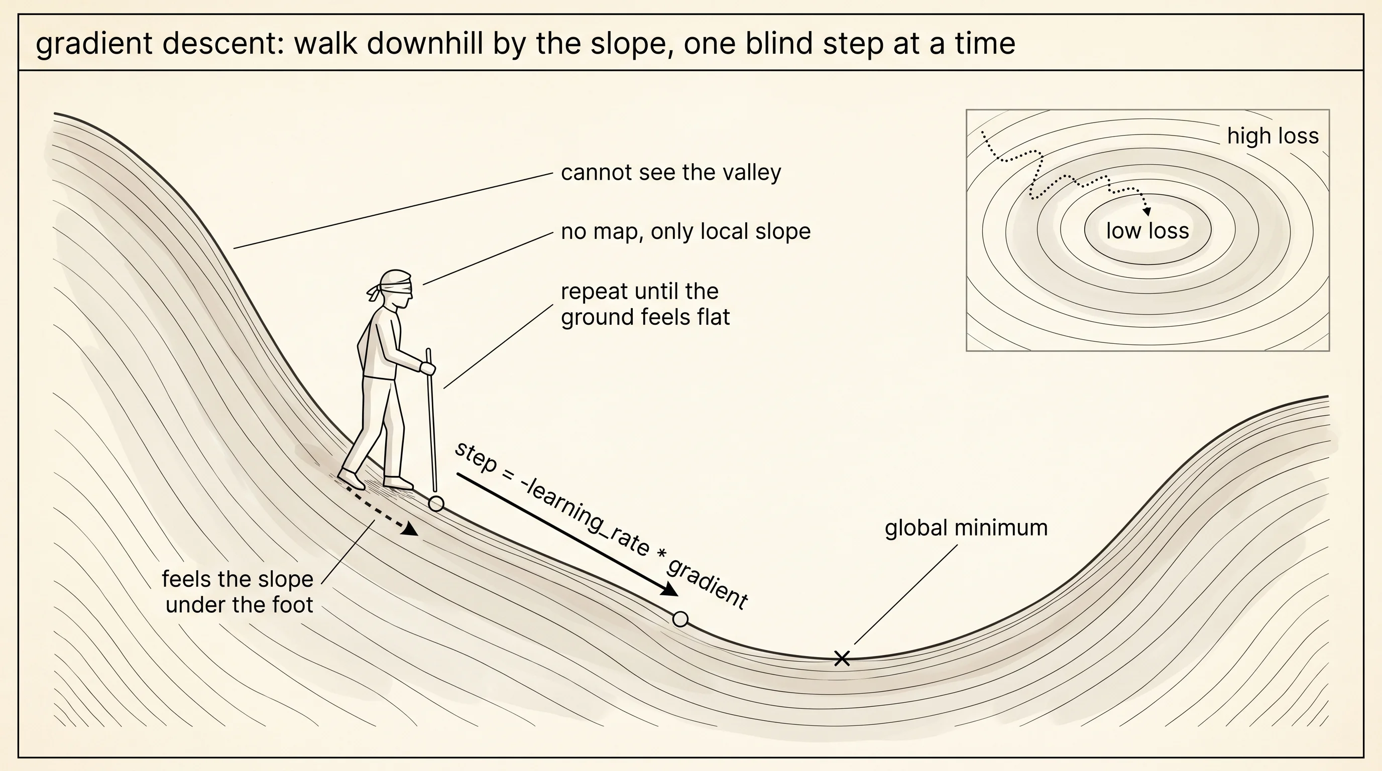
The slope of a loss surface has a name: the gradient. For a function of one variable the gradient is just the derivative — the slope of the line tangent to the curve at the current point. For a function of two variables the gradient is a pair, (df/dx, df/dy), which together point in the direction the surface climbs the fastest. Negate that pair and you have the direction of fastest descent. Multiply the negated gradient by a small number called the learning rate and you have a step. Add the step to the current point and you have the next point. That is the entire algorithm. Three lines.

# theta_next = theta - learning_rate * gradient_at(theta)

The hiker still has to compute the gradient somehow. The principled way is calculus — write the loss as a function, take partial derivatives by hand, plug in the current point. That works for a quadratic. It does not work for a Rosenbrock valley you wrote on a napkin five minutes ago. The lazy way that always works is finite differences. Step a tiny amount h to the right, evaluate the function, step a tiny amount h to the left, evaluate again. The difference divided by 2h is a clean estimate of the slope at the original point. Two function evaluations per partial. Slow, but you do not have to think.

def numerical_gradient(f, x, y, h=1e-5):
    dx = (f(x + h, y) - f(x - h, y)) / (2.0 * h)
    dy = (f(x, y + h) - f(x, y - h)) / (2.0 * h)
    return dx, dy

This is the central difference — the symmetric one. The naive forward difference would be (f(x + h) - f(x)) / h, which is fine but wrong by an amount proportional to h. Centering the step cancels that linear error and leaves a residue proportional to h * h, which at h = 1e-5 is one part in 10 billion. Good enough for any descent that does not need machine precision.

With the gradient in hand, the loop is direct. Start at a point, compute the gradient, step opposite it, repeat for a fixed number of steps, and keep the whole trail so you can look at it afterward.

def gradient_descent(f, x0, y0, lr, steps):
    path = [(x0, y0)]
    x, y = x0, y0
    for _ in range(steps):
        dx, dy = numerical_gradient(f, x, y)
        x -= lr * dx
        y -= lr * dy
        path.append((x, y))
    return path

Test it on the easiest surface that exists: a clean elliptical bowl, f(x, y) = x*x + y*y. The minimum is the origin. The gradient at any point (x, y) is (2x, 2y), which points straight away from the center. Negate it and every step from anywhere on the bowl marches directly at the bottom.

def quadratic(x, y):
    return x * x + y * y
 
path = gradient_descent(quadratic, x0=-1.8, y0=1.5, lr=0.1, steps=40)

To watch the descent, render the bowl as a contour map and overlay the path. Loss values get binned into four shading bands using the Unicode block characters ░ ▒ ▓ █ — light for low loss, heavy for high. The starting point shows up as S, the final point as E, and every cell the path passes through in between as *. The cells the path never touches keep their loss-shading.

███▓▓▓▓▒▒▒▒▒▒▒▒▒▒▒▓▓▓▓███
██▓▓▓▒▒▒▒▒▒▒▒▒▒▒▒▒▒▒▓▓▓██
█▓▓▓▒▒▒▒▒░░░░░░░▒▒▒▒▒▓▓▓█
▓S▓▒▒▒▒░░░░░░░░░░░▒▒▒▒▓▓▓
▓▓▒▒▒░░░░░░░░░░░░░░░▒▒▒▓▓
▓▒▒*░░░░░░     ░░░░░░▒▒▒▓
▓▒▒▒░*░░         ░░░░▒▒▒▓
▒▒▒░░░*           ░░░░▒▒▒
▒▒▒░░░  *          ░░░▒▒▒
▒▒░░░░  *          ░░░░▒▒
▒▒░░░    **         ░░░▒▒
▒▒░░░      *        ░░░▒▒
▒▒░░░      *E       ░░░▒▒
▒▒░░░               ░░░▒▒
▒▒░░░               ░░░▒▒
▒▒░░░░             ░░░░▒▒
▒▒▒░░░             ░░░▒▒▒
▒▒▒░░░░           ░░░░▒▒▒
▓▒▒▒░░░░         ░░░░▒▒▒▓
▓▒▒▒░░░░░░     ░░░░░░▒▒▒▓
▓▓▒▒▒░░░░░░░░░░░░░░░▒▒▒▓▓
▓▓▓▒▒▒▒░░░░░░░░░░░▒▒▒▒▓▓▓
█▓▓▓▒▒▒▒▒░░░░░░░▒▒▒▒▒▓▓▓█
██▓▓▓▒▒▒▒▒▒▒▒▒▒▒▒▒▒▒▓▓▓██
███▓▓▓▓▒▒▒▒▒▒▒▒▒▒▒▓▓▓▓███

The path is a near-straight line from the upper-left edge of the bowl down to the empty white center. The bowl is so symmetric that the gradient at every point on the path points almost exactly at the minimum. Forty steps and the hiker is sitting in the hole. Bowl-shaped surfaces are the dream. Real loss surfaces are not bowls.

The classic test for an optimizer that is not a bowl is the Rosenbrock function — Howard Rosenbrock published it in 1960 to embarrass slow optimization methods. The shape is a long curved valley with a narrow floor. The minimum sits at (1, 1). The valley walls are steep. The valley floor curves. The gradient at almost every point on the surface points across the valley, not down it.

def rosenbrock(x, y):
    a = 1.0 - x
    b = y - x * x
    return a * a + 100.0 * b * b

Start descent at (-1.5, 1.5). Use a small learning rate of 0.001 because the surface has cliffs of slope 100 — anything bigger overshoots into the wall and bounces. Run for 2000 steps.

rosen_path = gradient_descent(rosenbrock, x0=-1.5, y0=1.5, lr=0.001, steps=2000)

The print moment for this lesson is the trace. Every step, print (x, y, loss). Watch the path crawl down the curved valley.

step    x          y          loss
   0  -1.50000  +1.50000  62.500000
   1  -1.04500  +1.65000  35.315635
   2  -1.27414  +1.53840  5.894854
   3  -1.22626  +1.55541  5.223601
   4  -1.24717  +1.54507  5.060480
   5  -1.23751  +1.54714  5.031143
   6  -1.24081  +1.54400  5.023161
   7  -1.23851  +1.54312  5.019418
   8  -1.23860  +1.54128  5.016436
   9  -1.23766  +1.53985  5.013595
  10  -1.23717  +1.53824  5.010779
  11  -1.23648  +1.53671  5.007967
  12  -1.23588  +1.53514  5.005155
  13  -1.23524  +1.53359  5.002342
  14  -1.23461  +1.53204  4.999528
  15  -1.23398  +1.53048  4.996713
  16  -1.23335  +1.52893  4.993898
  17  -1.23272  +1.52737  4.991082
  18  -1.23209  +1.52582  4.988264
  19  -1.23146  +1.52426  4.985446
  20  -1.23082  +1.52271  4.982627
  21  -1.23019  +1.52115  4.979807
  22  -1.22956  +1.51960  4.976986
  23  -1.22893  +1.51804  4.974165
  24  -1.22829  +1.51648  4.971342

Read the columns. Step 0 starts at loss 62.5. Step 1 hops to a different x with loss 35 — that is the first big plunge over the wall of the valley. Step 2 lands inside the floor at loss 5.9 and the loss column basically stops moving. From step 4 to step 24, the loss drops by 0.003 per step. Look at the x and y columns next to that. Twenty steps and x has shifted by 0.018, y by 0.029. The hiker is on the valley floor and the floor is nearly flat under him. He is taking inch-long shuffles toward (1, 1) and he has another 1900 steps to go before he is close. Two thousand steps later he ends at (0.654, 0.427) with loss 0.12 — better than 5.9, but still not at the bottom.

The contour with the path overlaid shows the same story in a picture.

 
 
      *
   S**
     *
░    **                 ░
░     *                 ░
░     **                ░
░░     *               ░░
░░     **       E      ░░
░░      **     **      ░░
▒░       **   **       ░▒
▒░░       *****       ░░▒
▒░░                   ░░▒
▒░░                   ░░▒
▒▒░░                 ░░▒▒
▓▒░░                 ░░▒▓
▓▒░░                 ░░▒▓
▓▒░░░               ░░░▒▓
▓▒▒░░               ░░░▒▓
▓▓▒░░░             ░░░▒▓▓
█▓▒░░░             ░░░▒▓█
█▓▒▒░░             ░░▒▒▓█
█▓▒▒░░░           ░░░▒▒▓█
█▓▓▒░░░░         ░░░░▒▓▓█

The hiker drops onto the curved white valley floor in two big steps, then crawls to the right along the floor. The path makes the bend. It does not get to the bottom. This is the central problem with vanilla gradient descent: on a curved valley, the gradient at the floor is tiny, the step size is therefore tiny, and the hiker spends the whole afternoon walking at one inch per step while the valley curves under him.

A saddle is worse. The function f(x, y) = x*x - y*y is a minimum along the x-axis and a maximum along the y-axis. The point (0, 0) is a saddle — gradient zero, but not a minimum. The brain wants to think it has finished. It has not.

def saddle(x, y):
    return x * x - y * y
 
saddle_path = gradient_descent(saddle, x0=0.8, y0=0.05, lr=0.1, steps=40)

Start at (0.8, 0.05) — slightly off the axis, which is the realistic case in a high-dimensional model where you never sit on any axis exactly. The descent slides down the bowl in x while sliding up the hill in -y. The negative gradient in y is 2y, and since the descent rule subtracts that, the y value grows away from zero exponentially. At step 40 the hiker has converged to x = 0 (the right thing to do for the bowl direction) but y = 73.5 and the loss is -5400. He fell off the saddle.

A multimodal surface adds the last failure mode: local minima. The function f(x, y) = 0.1*(x*x + y*y) + sin(x)*sin(y) is a wide bowl with a sinusoidal ripple printed on top. The global minimum is at the origin. There are three other valleys nearby. Where descent ends depends entirely on where it started.

def multimodal(x, y):
    return 0.1 * (x * x + y * y) + math.sin(x) * math.sin(y)

Run descent from each of four starting corners.

start (-1.5, -1.5): end (-0.000, -0.000) loss  0.0000
start (+1.5, -1.5): end (+1.298, -1.298) loss -0.5904
start (-1.5, +1.5): end (-1.298, +1.298) loss -0.5904
start (+1.5, +1.5): end (+0.000, +0.000) loss  0.0000

Two of the four starts end at the global minimum. Two end at local minima at loss -0.59, which is worse than the global value of 0 only because the sinusoidal ripple creates negative pockets where sin(x)*sin(y) < 0. The hiker has no way to know there is a deeper hole on the other side of the ridge — he can only feel the slope under his feet, and the slope under his feet says "stay here." Local minima are gradient descent's permanent enemy. Modern training mostly survives them by running enormous models in enormous dimensions where saddles are common but strict local minima are rare. The sinusoidal toy is a warning, not a representative.

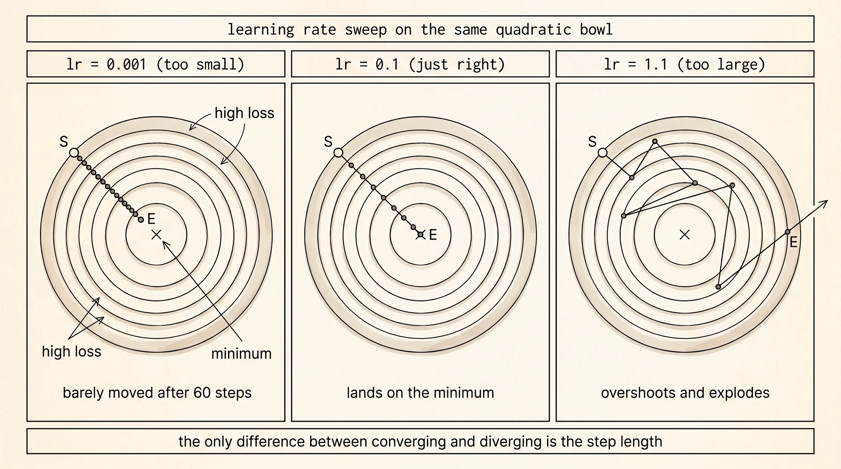
The other knob worth knowing how to break is the learning rate itself. Sweep it across the quadratic bowl from 0.001 to 1.1 and read the final loss in each row.

learning rate sweep on quadratic
    lr       end_x        end_y        end_loss
  0.0010   -1.59626    +1.33022    4.317549
  0.0100   -0.53560    +0.44633    0.486073
  0.1000   -0.00000    +0.00000    0.000000
  0.5000   +0.00000    +0.00000    0.000000
  0.9900   -0.53560    +0.44633    0.486073
  1.0100   -5.90586    +4.92155    59.100745
  1.1000   -101425.94840    +84521.34586    17431080914.407097

At lr = 0.001 the hiker has barely moved after 60 steps — he is still at loss 4.3 and his feet have not really left the start. At lr = 0.01 he is closer but not done. At lr = 0.1 and lr = 0.5 he lands on the minimum. At lr = 0.99 he is back to where lr = 0.01 was — the step is so close to the critical size that the hiker bounces back and forth across the valley and ends up the same distance away, on the other side. At lr = 1.01 the bouncing amplifies; each step throws him farther from the center than the last. By lr = 1.1 the position has exploded to coordinates of -101425, 84521 and the loss is 17 billion. Same surface, same start, same algorithm. The only difference is the step length.

A small question. Why does the quadratic bowl converge at exactly lr = 0.5 but diverge above lr = 1.0? The gradient of x*x + y*y at the point x is 2x. The update is x_new = x - lr * 2x = (1 - 2*lr) * x. The point gets multiplied by (1 - 2*lr) every step. If that factor has absolute value less than 1, the point shrinks toward zero — convergence. At lr = 0.5 the factor is exactly zero and the hiker lands on the minimum in one step. At lr = 1.0 the factor is -1 and the hiker bounces between x and -x forever. Above lr = 1.0 the factor exceeds 1 in absolute value and the position grows without bound. Every loss surface has its own critical learning rate. Cross it and the algorithm explodes.

Vanilla gradient descent crawls on hard terrain. The fix is to remember where you have been.