Learned Convolution

Padding lets the convolution survive the borders. The kernel itself, though, is still a fixed list of nine numbers picked by a human. Hand a 3x3 of negative-zero-positive rows to the picture and it fires on horizontal edges. Hand it a 3x3 average and it blurs. Somebody had to know what they wanted before they wrote the kernel down. An apprentice inspector at a bottling plant starts with no checklist at all. On day one she walks the line and circles defects at random. Her supervisor tells her every time she missed and every time she false-alarmed. After a week she has scribbled her own checklist, and after a thousand crates the checklist matches what the senior inspector has been carrying around for thirty years. She was never told what a defect looks like. She figured it out from the feedback.

The math of convolution is older than computers. Pierre-Simon Laplace and Jean-Baptiste-Joseph Fourier worked it out for differential equations in the 19th century — sliding one function across another and integrating the product was already the standard tool for blurring a noisy signal by 1900. Kunihiko Fukushima, a researcher at NHK Broadcasting Science Research Laboratory in Tokyo, built the first neural network shaped like the visual cortex in 1980. He called it the Neocognitron. It used convolutions, but the kernel weights were fixed by hand to detect lines and arcs the way the simple cells of a cat's visual cortex did. Yann LeCun, working at Bell Labs in 1989, saw what was missing. The same backpropagation that trained the weights of a regular neuron could train the nine numbers inside a 3x3 kernel. He plugged convolutions into a network that read handwritten zip codes off envelopes for the U.S. Postal Service, let gradient descent find the weights, and the kernels that came out were exactly the edge detectors Fukushima had typed in by hand — but discovered, not designed. The trick sat quietly for two decades. In 2012, Alex Krizhevsky in Geoffrey Hinton's lab in Toronto wrote the convolution loop on a pair of NVIDIA GTX 580 gaming GPUs in his bedroom, scaled the network to eight layers and 60 million parameters, and won the ImageNet contest by a margin that broke the field open. The kernels he printed at the end of training looked like color blobs and oriented edges — the same primitives a neuroscientist had recorded from the V1 visual cortex of a macaque in 1959.

To get a kernel to learn, the gradient has to flow through the convolution. Convolution itself is one nested loop — for every output position, sum the kernel weights times the matching pixels. The gradient with respect to one weight in the kernel is the sum, over every output position, of the upstream gradient at that position times the input pixel that the weight multiplied. Write it once, ship it forever — every CNN ever trained uses the same shape of expression.

def convolve_2d(image, kernel):
    image_h = len(image)
    image_w = len(image[0])
    kernel_h = len(kernel)
    kernel_w = len(kernel[0])
    out_h = image_h - kernel_h + 1
    out_w = image_w - kernel_w + 1
    output = [[0.0 for _ in range(out_w)] for _ in range(out_h)]
    for out_row in range(out_h):
        for out_col in range(out_w):
            total = 0.0
            for k_row in range(kernel_h):
                for k_col in range(kernel_w):
                    total += kernel[k_row][k_col] * image[out_row + k_row][out_col + k_col]
            output[out_row][out_col] = total
    return output
 
 
def convolve_2d_gradient(upstream_grad, input_image, kernel):
    kernel_h = len(kernel)
    kernel_w = len(kernel[0])
    out_h = len(upstream_grad)
    out_w = len(upstream_grad[0])
    grad_kernel = [[0.0 for _ in range(kernel_w)] for _ in range(kernel_h)]
    for k_row in range(kernel_h):
        for k_col in range(kernel_w):
            total = 0.0
            for out_row in range(out_h):
                for out_col in range(out_w):
                    total += upstream_grad[out_row][out_col] * input_image[out_row + k_row][out_col + k_col]
            grad_kernel[k_row][k_col] = total
    return grad_kernel

Read the gradient function. Outer loop walks the nine kernel weights. Inner loop walks the output. For each weight, the formula sums upstream gradient times the input pixel that lined up with that weight. This is the exact same nested loop as the forward pass, with the kernel weight replaced by the upstream gradient and the output replaced by the kernel-weight gradient. The convolution is its own backward pass — symmetric on the inside.

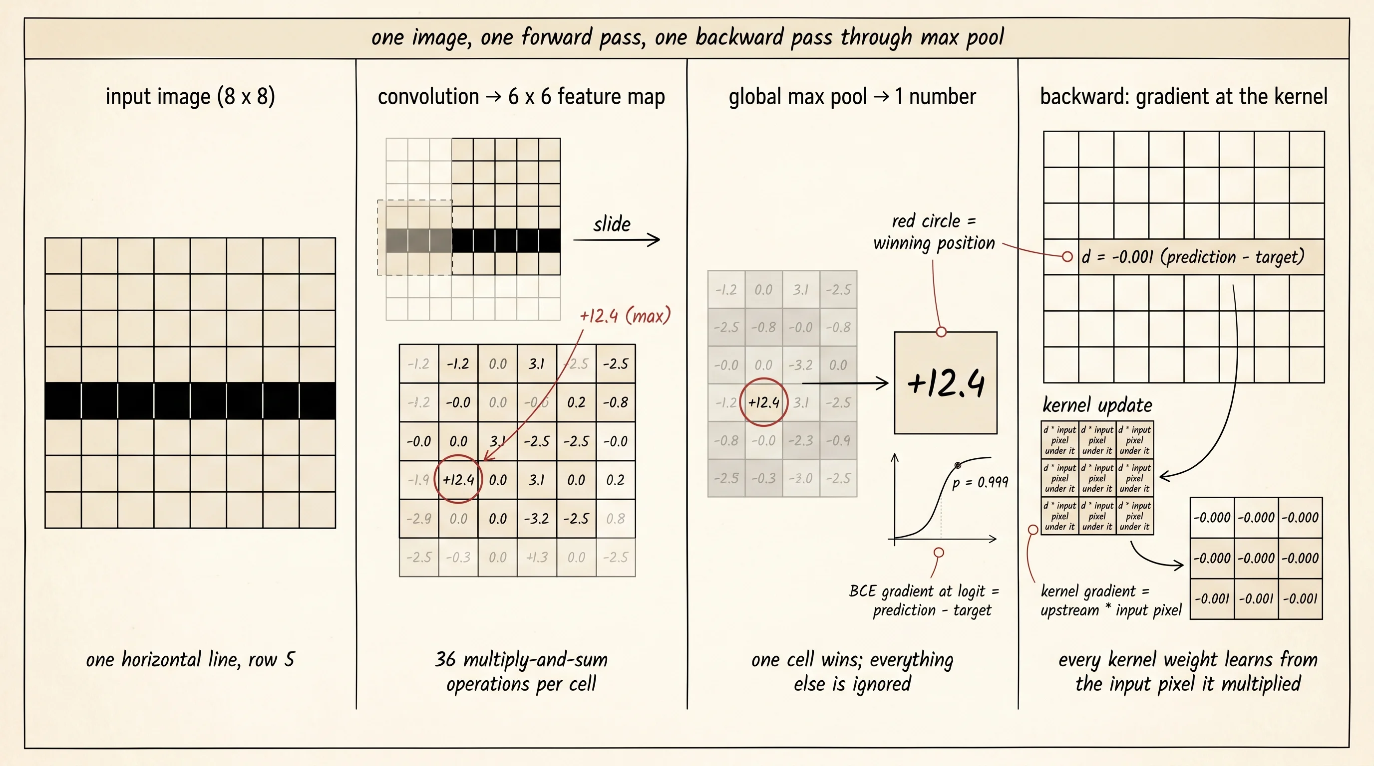
The data is two kinds of 8x8 picture: a horizontal line at some random row, or a vertical line at some random column. The lit pixels are 1.0, the dark pixels are 0.0. The job is one bit: did this picture have a horizontal line, or a vertical one?

import random
 
def generate_line_images(n, direction):
    images = []
    for _ in range(n):
        grid = [[0.0 for _ in range(8)] for _ in range(8)]
        if direction == "horizontal":
            row = random.randint(1, 6)
            for col in range(8):
                grid[row][col] = 1.0
        else:
            col = random.randint(1, 6)
            for row in range(8):
                grid[row][col] = 1.0
        images.append(grid)
    return images

The classifier is the simplest thing that can possibly learn this. One 3x3 kernel is convolved across the image, which leaves a 6x6 feature map. A global max pool collapses the feature map to one number — the strongest activation anywhere in the image. That number plus a bias goes through a sigmoid to become a probability, and the probability is compared to the label with binary cross-entropy. Three operations, two parameters that matter (the nine kernel weights and the bias).

import math
 
def sigmoid(x):
    if x > 50:
        return 1.0
    if x < -50:
        return 0.0
    return 1.0 / (1.0 + math.exp(-x))
 
 
def global_max_pool(feature_map):
    best_value = feature_map[0][0]
    best_row, best_col = 0, 0
    for row, values in enumerate(feature_map):
        for col, value in enumerate(values):
            if value > best_value:
                best_value = value
                best_row, best_col = row, col
    return best_value, best_row, best_col

The gradient through max pool is the punchline of this whole lesson. The max pool picks one cell out of the 36 cells in the 6x6 feature map and forwards its value. Every other cell is ignored. So the upstream gradient at the chosen cell is whatever sigmoid-and-loss hand back, and the upstream gradient at every other cell is exactly zero. The kernel only learns from the position where it fired hardest. Sigmoid plus binary cross-entropy collapses on the same shape of math as softmax plus categorical cross-entropy from a few lessons ago — the gradient at the logit is prediction minus target. One subtraction.

def train_step(kernel, bias, image, label, learning_rate):
    feature_map = convolve_2d(image, kernel)
    max_value, max_row, max_col = global_max_pool(feature_map)
    logit = max_value + bias
    prediction = sigmoid(logit)
    d_logit = prediction - label
 
    upstream = [[0.0 for _ in range(len(feature_map[0]))] for _ in range(len(feature_map))]
    upstream[max_row][max_col] = d_logit
 
    grad_kernel = convolve_2d_gradient(upstream, image, kernel)
    for k_row in range(3):
        for k_col in range(3):
            kernel[k_row][k_col] -= learning_rate * grad_kernel[k_row][k_col]
    new_bias = bias - learning_rate * d_logit
    return new_bias

The training loop draws a coin to decide horizontal or vertical, generates one image of that kind, runs train_step, and prints the kernel every 100 steps. The kernel starts as nine random numbers picked from a Gaussian. After 100 updates it has the rough shape. After 600 updates it is a horizontal-edge detector with no human in the loop.

random.seed(7)
 
kernel = [[random.gauss(0.0, 0.3) for _ in range(3)] for _ in range(3)]
bias = 0.0
 
print("initial kernel (random):")
for row in kernel:
    print("  " + " ".join(f"{value:+.3f}" for value in row))
 
for step in range(600):
    if random.random() < 0.5:
        label = 1.0
        image = generate_line_images(1, "horizontal")[0]
    else:
        label = 0.0
        image = generate_line_images(1, "vertical")[0]
    bias = train_step(kernel, bias, image, label, learning_rate=0.1)
    if (step + 1) % 100 == 0:
        print(f"\nstep {step + 1}:")
        for row in kernel:
            print("  " + " ".join(f"{value:+.3f}" for value in row))

Run it and watch the kernel resolve.

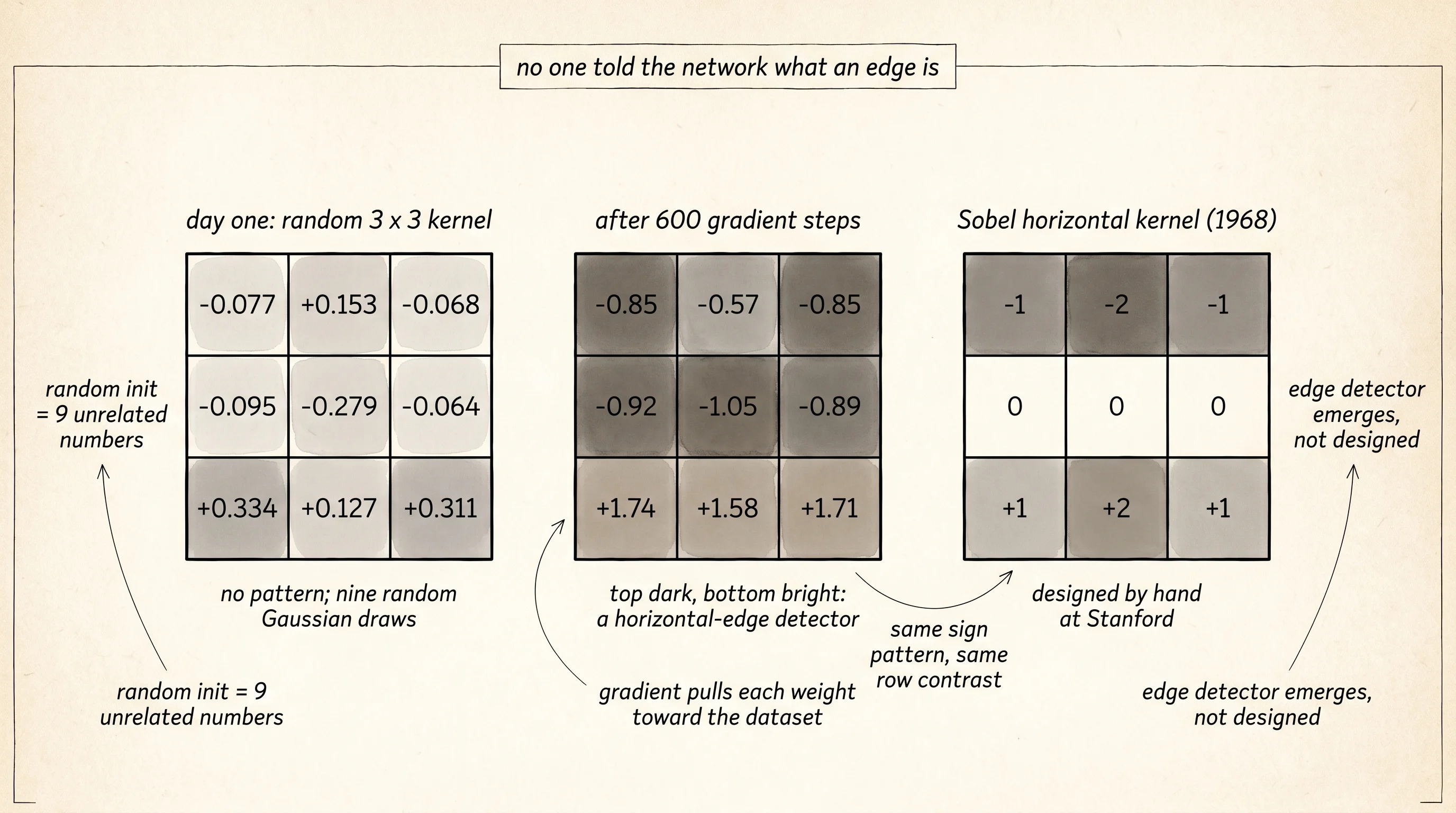
initial kernel (random):
  -0.077 +0.153 -0.068
  -0.095 -0.279 -0.064
  +0.334 +0.127 +0.311
 
step 100:
  -0.447 -0.163 -0.440
  -0.514 -0.646 -0.486
  +0.867 +0.714 +0.842
 
step 200:
  -0.572 -0.310 -0.588
  -0.639 -0.792 -0.634
  +1.224 +1.050 +1.176
 
step 400:
  -0.762 -0.477 -0.758
  -0.830 -0.960 -0.804
  +1.529 +1.377 +1.502
 
step 600:
  -0.849 -0.565 -0.845
  -0.917 -1.047 -0.891
  +1.737 +1.584 +1.709

Read the final kernel one row at a time. The top row is strongly negative. The middle row is strongly negative. The bottom row is strongly positive. Slide that pattern across an image and it fires hardest exactly when the bottom row of the kernel sits on a bright stripe and the rows above sit on dark pixels — which is the bottom edge of a horizontal line. It fires negatively when a vertical line cuts through the kernel's middle column, because the middle column has all-negative weights. The shape is unmistakable. Compare it to the Sobel horizontal-edge kernel from the last lesson:

sobel horizontal:        learned kernel:
-1  -2  -1               -0.85  -0.57  -0.85
 0   0   0               -0.92  -1.05  -0.89
+1  +2  +1               +1.74  +1.58  +1.71

Same sign pattern. Same row contrast. Irwin Sobel published his kernel in 1968. Yann LeCun's network discovered the same kernel from a few hundred examples in 1989. Nobody told the network what a horizontal edge is. The network found out because gradient descent on prediction minus target pulled every weight in the direction that lowers the loss, and the only setting of the nine weights that lowers the loss on this dataset is the setting that detects horizontal edges.

A small question. Why does the middle row of the learned kernel come out close to zero in Sobel but strongly negative here? Because the data is different. Sobel was designed for natural images where edges are rarely a single pixel thick — a real edge has gradient on both sides of it, so the middle row should not commit to a sign. The lines in this dataset are exactly one pixel thick. The kernel that wins on this data uses the middle row as a second negative band so that a vertical line passing under the kernel scores even more negative. The gradient does not do what a textbook would do. It does what the data demands.

Every convolution at full resolution is expensive, and the next move is to trade pixels for compute by skipping positions instead of visiting all of them.