Dilated Convolutions

A pair of bifocals sits on the desk. The top lens is a normal pane and reads the page right under the nose. The bottom lens is the same width — same number of glass elements — but ground so that each element samples the page at twice the spacing. Look through the top and the kernel sees pixels 0, 1, 2. Look through the bottom and the same three taps see pixels 0, 2, 4. Stack a third lens and the taps see 0, 4, 8. The hand on the rim never moves. The number of pieces of glass never changes. The patch of paper in focus doubles every time another lens slips into the frame. That is the trick that lets a convolutional network read a whole sentence, a whole second of audio, or a whole image with a stack only 5 layers deep.

Fisher Yu and Vladlen Koltun published the trick in 2016 in Multi-Scale Context Aggregation by Dilated Convolutions. They were trying to label every pixel in a street photo as road, car, sky, or person — semantic segmentation, where the answer at the center pixel depends on the boundaries 100 pixels away. Stacking ordinary 3x3 convolutions worked but cost a forest of layers, and every layer of pooling that grew the receptive field also threw away the spatial detail the segmenter needed. Dilation gave them coverage without downsampling. A few months later Aäron van den Oord and the team at DeepMind shipped WaveNet, which generated raw 16,000-sample-per-second audio one sample at a time by stacking causal dilated convolutions with dilations [1, 2, 4, 8, ..., 512] and then doing it again for ten more blocks. The receptive field reached back thousands of samples — enough to remember the shape of a syllable — with the parameter count of a small image network. The same receptive-field idea echoes through the state-space architectures Albert Gu and Tri Dao introduced as Mamba in 2023, where a recurrence is engineered to look back exponentially far without a quadratic attention bill.

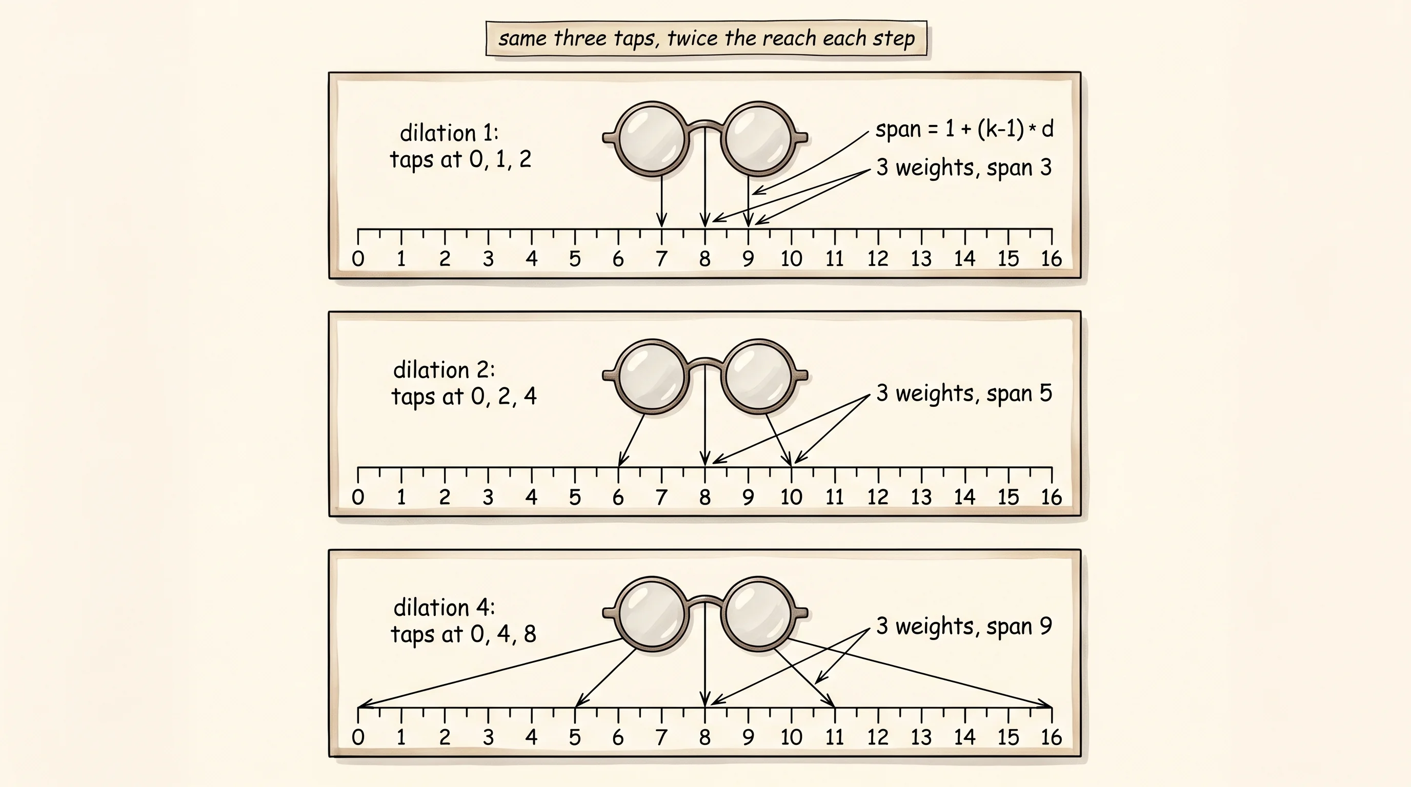
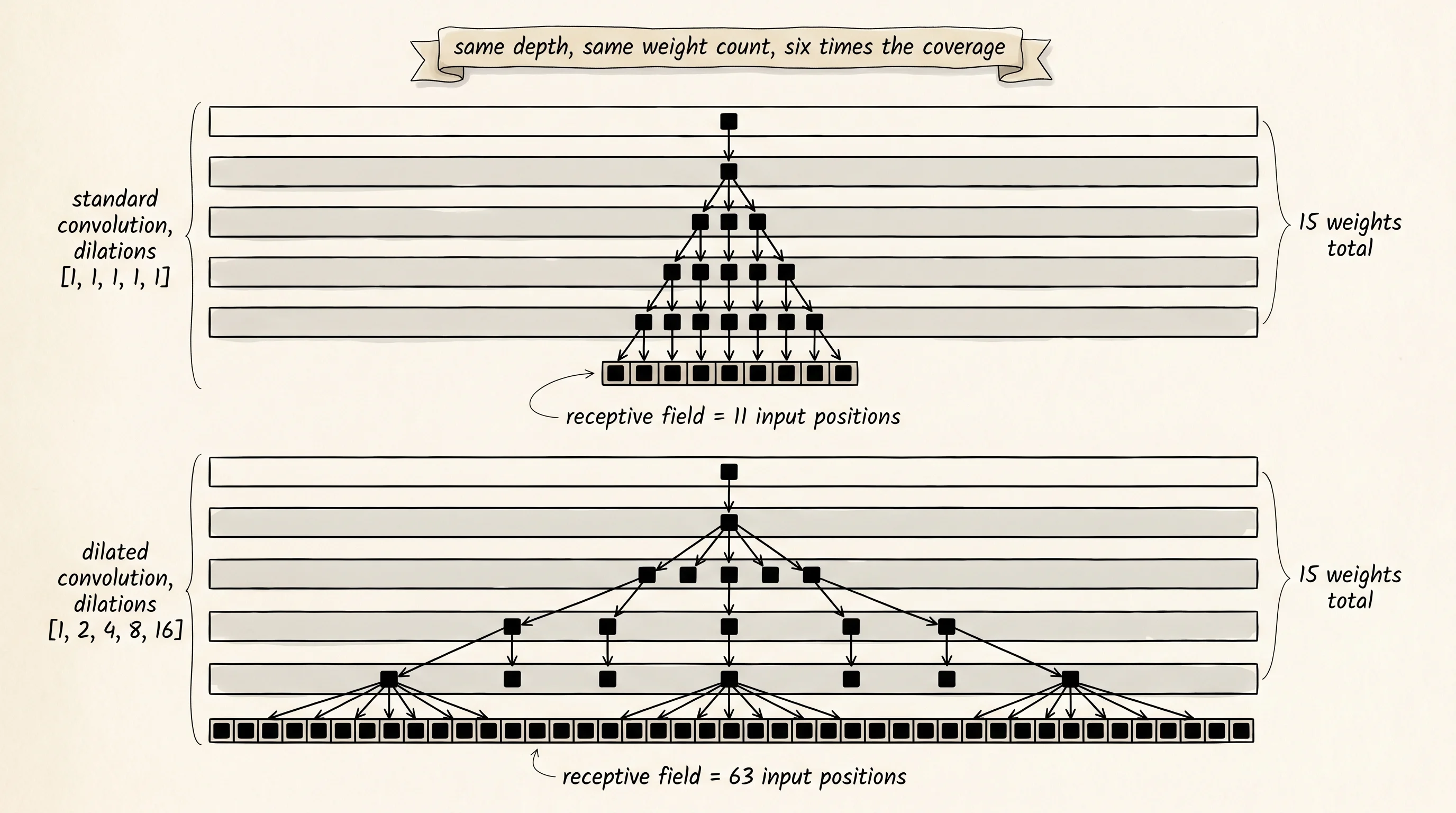
The math is two lines. A standard convolution with kernel size k and dilation 1 reads positions [i, i+1, i+2, ..., i+k-1] of its input. Dilation d spreads the taps: it reads [i, i+d, i+2d, ..., i+(k-1)d]. The kernel still has k weights. The span of the input it touches grows from k to 1 + (k-1)_d. Stack n layers of kernel size k with dilations d_1 through d_n and the receptive field at the top of the stack is 1 + (k-1) _ (d_1 + d_2 + ... + d_n). With kernel 3 and a doubling schedule [1, 2, 4, 8, 16], the sum is 31, the receptive field is 63, and the weight count is 5 * 3 = 15. The same coverage with standard kernel-3 layers would need 31 layers and 93 weights. Two thirds of the parameters disappear, and 26 layers' worth of intermediate activations along with them.

Open main.py and write the slide. The signal is a list of floats. The kernel is a shorter list of floats. The output position at index i is the sum of kernel[t] * signal[i + t * dilation] for every tap index t. The valid output length is len(signal) - (kernel_size - 1) * dilation — the number of starting positions where every tap still lands inside the signal.

def dilated_convolve_1d(signal, kernel, dilation):
    kernel_size = len(kernel)
    span = (kernel_size - 1) * dilation
    output_length = len(signal) - span
    output = []
    for output_index in range(output_length):
        total = 0.0
        for tap_index in range(kernel_size):
            signal_index = output_index + tap_index * dilation
            total += kernel[tap_index] * signal[signal_index]
        output.append(total)
    return output

Run it on a signal that alternates between a number and a zero, with an all-ones kernel. The dilation-1 pass reads three consecutive samples and so always sums one zero and two non-zeros. The dilation-2 pass skips the zeros entirely and sees only the non-zeros — the same three taps now sample 1, 2, 3 instead of 1, 0, 2.

signal = [1.0, 0.0, 2.0, 0.0, 3.0, 0.0, 4.0, 0.0, 5.0]
kernel = [1.0, 1.0, 1.0]
print(dilated_convolve_1d(signal, kernel, dilation=1))
print(dilated_convolve_1d(signal, kernel, dilation=2))

[3.0, 2.0, 5.0, 3.0, 7.0, 4.0, 9.0]
[6.0, 0.0, 9.0, 0.0, 12.0]

The dilation-2 row reads [1+2+3, 0+0+0, 2+3+4, 0+0+0, 3+4+5] and you can see the kernel walking past the zeros with a stride that perfectly skips them. The receptive field of the second row is 5 input samples per output, where the first row's was 3.

Add the analytical receptive-field calculator. The recurrence is the line above written in code: start at 1 and add (kernel_size - 1) * dilation for every layer.

def compute_receptive_field(n_layers, kernel_size, dilations):
    receptive_field = 1
    for layer_index in range(n_layers):
        receptive_field += (kernel_size - 1) * dilations[layer_index]
    return receptive_field

To draw which input positions actually feed the output, walk the dependency graph backward. Start with one position at the top. At each layer below, replace every position with the k positions its kernel reads, spaced by that layer's dilation. After n steps the set of positions you have collected is the receptive field as a concrete set of indices.

def trace_dependencies(n_layers, kernel_size, dilations):
    positions = {0}
    for layer_index in reversed(range(n_layers)):
        dilation = dilations[layer_index]
        next_positions = set()
        for position in positions:
            for tap_index in range(kernel_size):
                next_positions.add(position + tap_index * dilation)
        positions = next_positions
    return sorted(positions)
 
 
def visualize_receptive_field(n_layers, kernel_size, dilation):
    dilations = [dilation] * n_layers if isinstance(dilation, int) else list(dilation)
    receptive_field = compute_receptive_field(n_layers, kernel_size, dilations)
    touched = set(trace_dependencies(n_layers, kernel_size, dilations))
    return "".join("█" if p in touched else "." for p in range(receptive_field))

Stack 5 standard layers and 5 dilated layers and print the layer-5 receptive field of each, side by side.

standard = visualize_receptive_field(n_layers=5, kernel_size=3, dilation=1)
dilated = visualize_receptive_field(n_layers=5, kernel_size=3, dilation=[1, 2, 4, 8, 16])
print(f"standard ({len(standard):>2}): {standard}")
print(f"dilated  ({len(dilated):>2}): {dilated}")

standard (11): ███████████
dilated  (63): ███████████████████████████████████████████████████████████████

11 pixels versus 63 pixels. Same kernel size, same number of layers, same total weight count (15 weights in each stack). The standard row is what the network at the top of a 5-layer plain CNN can see when it makes a decision about the center pixel. The dilated row is what the same-size network sees with the dilation schedule slipped in. The difference is not a small efficiency win. It is the difference between recognizing a syllable and recognizing a word, between seeing a brake light and seeing the car the brake light belongs to.

A small question. Why does the dilated row come out solid instead of striped — when dilation 16 means the kernel reads positions 16 apart, shouldn't the row have gaps every few pixels? Because the lower layers fill in the gaps that the higher layers leave. Dilation 16 at the top reads positions 0, 16, 32. Each of those positions is the output of a layer with dilation 8, which reads three positions 8 apart. Those in turn are outputs of dilation 4, then dilation 2, then dilation 1. The doubling schedule was chosen exactly so the holes from layer n are covered by the wider span of layer n+1. Pick a non-doubling schedule like [1, 4, 8] and the row comes out as ███.███.███.███.███.███.███ — Yu and Koltun called the dotted gaps gridding artifacts and showed them ruining segmentation outputs in the same paper that introduced the technique. The doubling sequence is not a guess. It is the only schedule that grows the field exponentially without leaving holes.

You have built convolutional networks from scratch. Real-world tasks rarely have enough data to train one from zero.