Pooling and Shift Invariance

A security guard stands at the end of a hallway and a detective walks up. The detective does not ask "where exactly was the suspect standing in tile 47, column 3 of the floor." The detective asks "did you see anyone matching this description in this hallway." The guard scans the hallway, picks the strongest match, and answers yes or no. The exact tile gets thrown away on purpose. That throwaway is what makes the answer survive a person who shifted one step left between the time the report was filed and the time the guard looked up. Pooling is the same trick wired into a convolutional network. After the kernel slides across the picture and writes one match score per position, a pool window collapses every small neighborhood into its strongest score. The exact pixel where the match landed is gone. The fact that a match landed somewhere nearby is preserved.

Kunihiko Fukushima at NHK Broadcasting Science Research Laboratory in Tokyo built the first version in 1980 and called it the Neocognitron. His network had two kinds of layers wired in alternation — one shaped like the simple cells in a cat's visual cortex that fired on oriented edges, and one shaped like the complex cells that fired on the same edge no matter where the cat moved its eyes. The complex-cell layer was the first pooling layer. Yann LeCun took the same skeleton to Bell Labs in 1989 and built LeNet, the network the U.S. Postal Service used to read handwritten zip codes. LeNet pooled by averaging — every 2x2 block of activations was replaced by its mean. Average pooling held for 20 years. Then in 2010 Dominik Scherer, Andreas Müller, and Sven Behnke at the University of Bonn ran a head-to-head test on object recognition and showed max pooling beat average pooling on every benchmark they ran. The reasoning was that max kept the strongest piece of evidence in the window and threw the noise out, while average diluted the evidence with everything around it. Four years later Min Lin, Qiang Chen, and Shuicheng Yan at the National University of Singapore wrote Network in Network and pushed the idea to its limit — replace the entire stack of fully connected layers at the end of a CNN with a single global average pool that collapses each feature map down to one number. GoogLeNet picked it up in 2014 and ResNet locked it in for every architecture that followed.

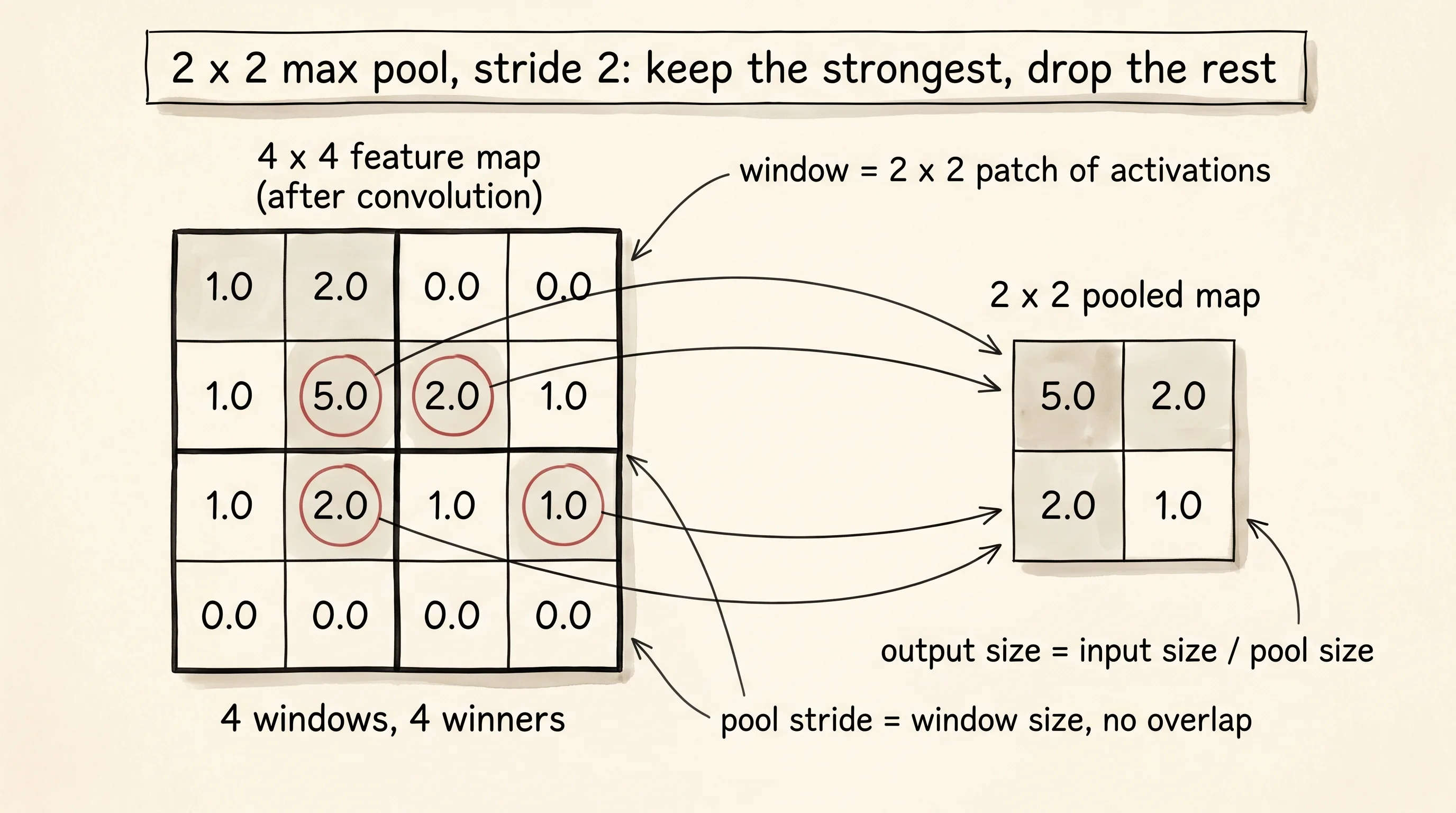
The math is one window at a time. Walk a pool_size by pool_size window across the feature map with a stride equal to pool_size so the windows do not overlap. Inside each window keep the largest value and write it into the output. A 6x6 feature map with a 2x2 max-pool comes out 3x3 — height and width both divided by the pool size. No weights, no learning, no parameters. The only choice the architect makes is the size of the window.

Build it. Open projects/21-shift-invariant-pattern-matcher/main.py. The image is a 2D list of floats. The template is a smaller 2D list. Convolution slides the template across the image and writes one activation per position — the sum of element-wise products between the template and the image patch under it.

def convolve(image, template):
    image_height = len(image)
    image_width = len(image[0])
    template_height = len(template)
    template_width = len(template[0])
    out_height = image_height - template_height + 1
    out_width = image_width - template_width + 1
    activation = [[0.0 for _ in range(out_width)] for _ in range(out_height)]
    for out_row in range(out_height):
        for out_col in range(out_width):
            total = 0.0
            for k_row in range(template_height):
                for k_col in range(template_width):
                    total += template[k_row][k_col] * image[out_row + k_row][out_col + k_col]
            activation[out_row][out_col] = total
    return activation

Max pool is 4 nested loops on top of that. Outer 2 loops walk the output cells. Inner 2 loops walk the pool window and track the largest value seen.

def max_pool(feature_map, pool_size):
    height = len(feature_map)
    width = len(feature_map[0])
    out_height = height // pool_size
    out_width = width // pool_size
    pooled = [[0.0 for _ in range(out_width)] for _ in range(out_height)]
    for out_row in range(out_height):
        for out_col in range(out_width):
            best = feature_map[out_row * pool_size][out_col * pool_size]
            for k_row in range(pool_size):
                for k_col in range(pool_size):
                    value = feature_map[out_row * pool_size + k_row][out_col * pool_size + k_col]
                    if value > best:
                        best = value
            pooled[out_row][out_col] = best
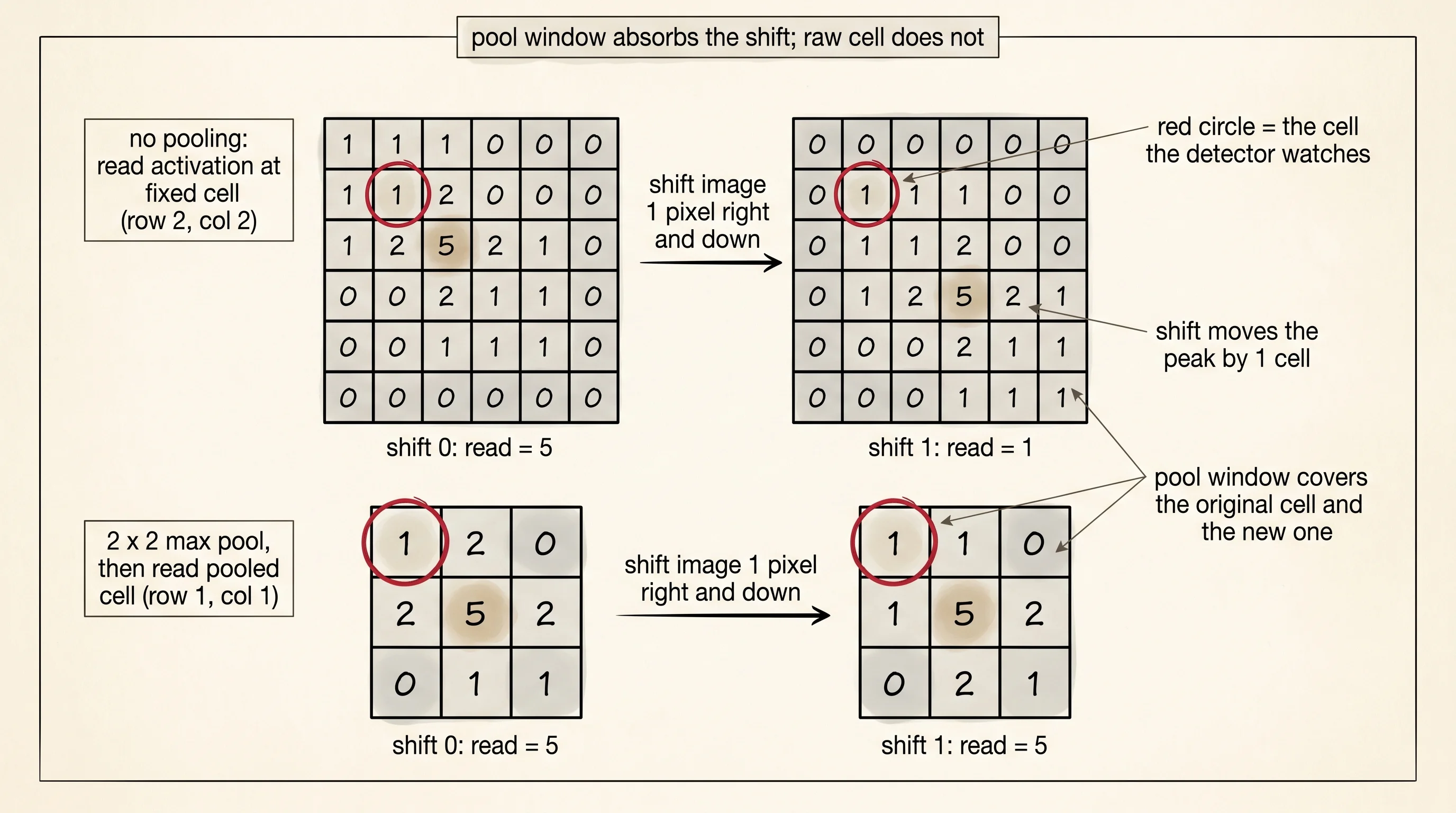
    return pooled

The smallest experiment that shows pooling earning its keep is an L-shaped template hunting an L-shaped pattern in an 8x8 image. Burn the L into the image at row 2, column 2. Cut a 3x3 L template. Convolve. The activation map peaks at exactly row 2, column 2 with a perfect score of 5 — five pixels in the L, every one of them lined up with a 1 in the template, sum is 5. Read that one cell and the detector says "match here, score 5." Then shift the image 1 pixel down and 1 pixel right. The L is still in the picture, just moved. Convolve again. The peak of 5 is still in the activation map, but now it has slid to row 3, column 3. Read row 2, column 2 again — the cell where the match used to be — and the score has collapsed.

Pool the activation map first, then read. A 2x2 max-pool over the 6x6 activation map gives a 3x3 pooled map where each cell holds the strongest match in its 2x2 window. The original peak at row 2, column 2 falls inside the pooled cell at row 1, column 1. After a 1-pixel shift the new peak at row 3, column 3 also falls inside that same pooled cell — different corner, same window. The pooled cell still reports 5. The detector does not care which corner.

Run the project and watch the numbers.

from main import make_image, place_l, l_template, detection_robustness_test
 
image = make_image(8, 8)
place_l(image, 2, 2)
template = l_template()
shifts = [0, 1, 2, 3]
 
raw = detection_robustness_test(image, template, shifts, pooling=False,
                                 pool_size=2, expected_row=2, expected_col=2)
pooled = detection_robustness_test(image, template, shifts, pooling=True,
                                   pool_size=2, expected_row=2, expected_col=2)
 
print(f"{'shift':>5}  {'no pool':>8}  {'2x2 max-pool':>13}")
for s, r, p in zip(shifts, raw, pooled):
    print(f"{s:>5}  {r:>8.1f}  {p:>13.1f}")

shift   no pool   2x2 max-pool
    0       5.0            5.0
    1       1.0            5.0
    2       1.0            1.0
    3       0.0            1.0

Read the table. At shift 0 both readouts give 5 — the match is exactly where the detector is looking. Shift the image by 1 pixel and the raw readout collapses from 5 to 1, because the peak slid out from under the cell the detector was watching. The pooled readout is still 5, because the peak only slid one cell over and that cell shares a pool window with the original. Shift by 2 and the pool window finally loses the peak, dropping to 1. Shift by 3 and the raw readout is 0 — the template no longer overlaps the L at the watched cell at all — while the pool still reports 1 from a partial overlap nearby. A 2x2 pool buys 1 pixel of shift tolerance for free. A 3x3 pool would buy 2. A network with three pooling layers stacked, each pooling 2x2, sees an effective tolerance of 8 pixels at the input — every pool layer doubles the size of a pixel in the layer above.

A small question. Why does the pooled score stay at 5 after a 1-pixel shift but not a 2-pixel shift? The pool window covers a 2x2 patch of activations. A 1-pixel shift moves the peak inside the same window. A 2-pixel shift moves the peak into the next window over, and the original window now sees only the 1's around the edges of the original L instead of the 5 at its center. Pooling smooths over shifts up to its window size. Beyond that, the next pool window catches the answer instead — which is why deep CNNs stack pooling layers and let each one cover a wider neighborhood than the one below it.

Pooling does this with no parameters at all. The convolution layer underneath it has 9 weights to learn. The pool layer on top of it has 0 weights — a fixed function that takes a window and returns its max. That is why average pooling lasted 20 years and max pooling replaced it overnight when Scherer's team showed the numbers. Nothing was being trained. The architect picked the function and the function did its job. Lin, Chen, and Yan took it one step further with global average pooling — instead of a 2x2 window, the window covers the entire feature map, collapsing a 7x7 spatial map into a single number per channel. The fully connected layer that used to live at the top of every CNN, holding 90 percent of the parameter count, was erased in one stroke. ResNet ships with global average pooling at the top to this day.

A 2x2 max pool with stride 2 cuts the spatial size in half. Stack 5 of them and the original 224x224 image is down to 7x7 by the time the network reads it out — the same arithmetic that justified strided convolutions in the previous lesson, but with no weights to train and no risk of the kernel learning to throw away the wrong information. Stride and pool both downsample. Stride does it while learning. Pool does it while letting position drift. The two tools coexist in every modern CNN.

Standard convolutions still have to grow their view of the image one pixel at a time per layer. There is a trick that grows the receptive field exponentially instead.