Transfer Learning

A boxer who switches to MMA does not start over. The footwork is already tuned. The conditioning is already there. The head movement, the distance management, the way he reads a flinch in his opponent's shoulders — every piece of that hardware was built across a thousand sparring rounds and it all carries forward. The grappling is new. The leg kicks are new. The cage takedowns are new. The smart move is to keep the boxer's coach for footwork and bolt on a wrestling coach for the new stuff. The dumb move is to fire the boxing coach, put the fighter back in pee-wee karate, and rebuild the entire athlete from the floor.

Jeff Donahue and a team at Berkeley wrote down the same trick for vision in 2014. Their paper was called DeCAF. They took an 8-layer convolutional network that Alex Krizhevsky had trained on ImageNet — 1.2 million labeled photos, the network that broke the field open in 2012 — and they did something nobody had bothered to try at scale. They froze the first 7 layers, threw away the final classification layer, and trained a single fresh classifier on top for a different task. Bird species. Scenes. Object attributes. Tasks where nobody had a million labeled examples. The network had never seen a bird in the right way for the new task and it still beat every system that had been hand-engineered for that task over the previous decade. A few months later Jason Yosinski, working with Yoshua Bengio at Montreal, ran the experiment that explained why. Layer 1 of a vision network is edges. Layer 2 is corners and color blobs. Layer 3 is textures. Those are the same on every photograph in the world — a wing, a bumper, a face, a leaf, all of them are stitched out of edges and textures. Only the top layers are task-specific. Howard and Ruder ported the same trick to text in 2018 with a system called ULMFiT. Google's BERT followed in 2019 and made "pretrain, then fine-tune" the default move for every language model since. The biggest models in the world today — GPT, Claude, Gemini — are all the boxer-to-MMA story at industrial scale: pretrain on the whole internet, then bolt on the task-specific head.

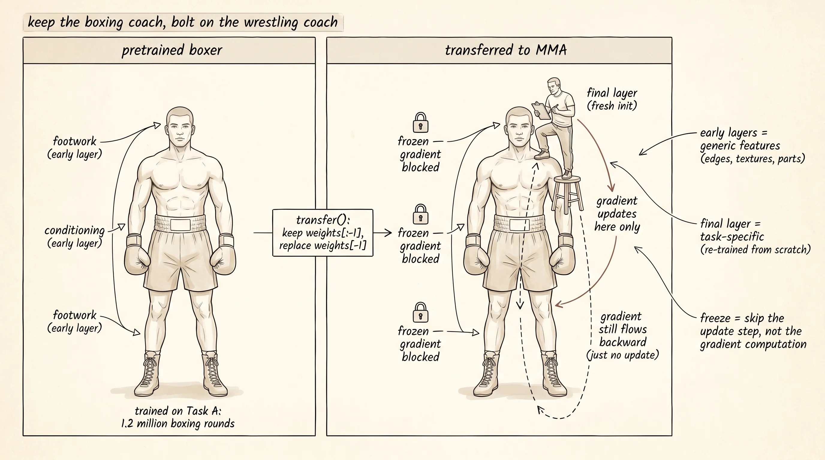
The cortex you have spent the last 4 lessons building from primitives — convolutions that learn edges, padding that protects the borders, pooling that earns shift-tolerance, dilation that grows the receptive field without growing the weight count — is now mature enough to inherit from another brain. The early layers are general. They live below the level of any one task. The trick of this lesson is to write the wiring that lets you take those early layers off one network and slot them into the next one with the parameters intact and the gradient pen lifted.

The project for this lesson is in projects/28-feature-reuse-experiment/main.py. The setup is the smallest controlled experiment that can show the gap. Task A is circle versus square on an 8x8 grid. Task B is triangle versus diamond on the same 8x8 grid. The architecture is a 3-layer MLP — 64 inputs into a 16-neuron hidden layer, into an 8-neuron hidden layer, into 1 sigmoid output. Read build_dataset and Network first. The shape function is plain geometry: a circle is the set of pixels within a radius of the center, a diamond is the set of pixels whose Manhattan distance from the center is at most the radius. The boxer is going to learn the first task, and the wrestling coach is going to be wired in on top for the second.

def transfer(pretrained_network, new_output_size):
    transferred = Network.__new__(Network)
    transferred.layer_sizes = list(pretrained_network.layer_sizes[:-1]) + [new_output_size]
    transferred.weights = list(pretrained_network.weights[:-1])
    transferred.biases = list(pretrained_network.biases[:-1])
    final_fan_in = pretrained_network.layer_sizes[-2]
    transferred.weights.append(init_weights(final_fan_in, new_output_size))
    transferred.biases.append(init_biases(new_output_size))
    frozen_layers = set(range(transferred.num_layers() - 1))
    return transferred, frozen_layers

Read this slowly. pretrained_network.weights[:-1] is "every weight matrix except the last one." Those matrices come across by reference — the new network points at the same memory the old one was using, so any update would change both. The final layer is brand new: a fresh weight matrix sized for the new output dimension and a fresh bias vector. frozen_layers names every layer except the new one. The freeze is enforced one layer up, inside apply_gradients:

def apply_gradients(network, weight_gradients, bias_gradients, learning_rate, frozen_layers):
    for layer_index in range(network.num_layers()):
        if layer_index in frozen_layers:
            continue
        # ... update weights and biases

Notice what is missing. The backward pass still runs through every layer. The early-layer gradients still get computed — they have to, because the next layer down needs them in its own gradient computation. The only thing the freeze does is skip the update step. The early features are protected because gradient descent never gets to push them around.

Run the project as it ships. From the project folder, python main.py. The default output is a flat line at the random-guess baseline:

 epoch   transferred   from scratch      gap
----------------------------------------------
     1         0.500          0.500   +0.000
     6         0.500          0.500   +0.000
   ...
    46         0.500          0.500   +0.000
----------------------------------------------
final          0.500          0.500   +0.000
 
transferred never crossed 90% accuracy
from scratch never crossed 90% accuracy (best = 0.500)

Both networks are stuck at 0.500 — the accuracy you would get by flipping a coin. This is not a transfer-learning failure. This is the dying-ReLU problem catching the network with the default LEARNING_RATE = 0.5 at the top of the file. The first gradient step is so big it pushes most of the hidden-layer pre-activations below zero, and once a ReLU sits at zero it has gradient zero and never wakes up. The whole network collapses to a constant output. A boxer cannot transfer technique to MMA if the boxer is unconscious.

Open main.py and change a single line near the top. LEARNING_RATE = 0.5 becomes LEARNING_RATE = 0.05. Save. Run again.

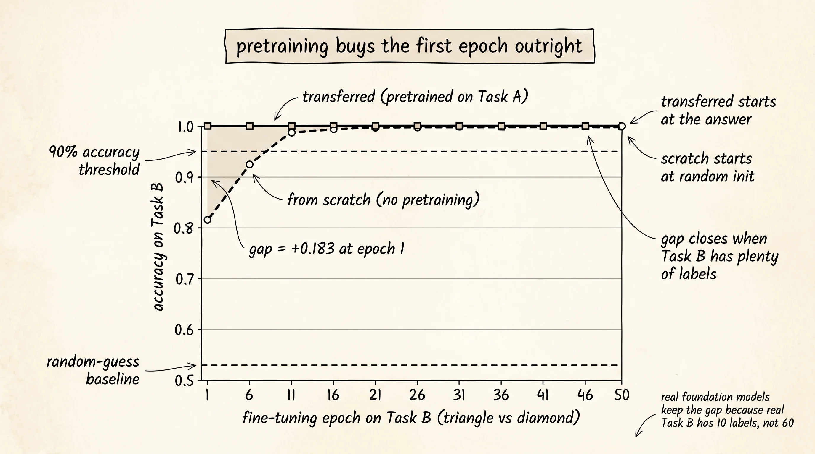
 epoch   transferred   from scratch      gap
----------------------------------------------
     1         1.000          0.817   +0.183
     6         1.000          1.000   +0.000
    11         1.000          1.000   +0.000
   ...
    46         1.000          1.000   +0.000
----------------------------------------------
final          1.000          1.000   +0.000
 
transferred crossed 90% accuracy at epoch 1
from scratch crossed 90% accuracy at epoch 2

The transferred network solves Task B on its first epoch — the gap at epoch 1 is +0.183, and the network is already at 100% accuracy. The from-scratch network needs a second epoch to catch up. In a head-to-head where the test was a single epoch of fine-tuning, the boxer-with-pretraining wins outright. The reason the gap closes by epoch 6 is that the data is too easy — 30 examples of a triangle versus 30 examples of a diamond is enough for either network to hit ceiling. Real transfer learning shows a permanent gap because real Task B has very few labels. The early-layer features the from-scratch network has to invent from 100 examples are the same features the pretrained network walked in with for free.

A small question. The from-scratch network has the same architecture, the same data, and runs the same number of epochs. Why does it lose the first epoch? Because its first hidden layer starts at random — a Gaussian of weights with no structure in them. The gradient on Task B has to walk those random weights into something that responds to triangle-and-diamond shapes. The transferred network's first layer starts at the configuration that already responds to circle-and-square shapes, which is mostly the configuration that responds to any 8x8 black-and-white shape. The early layer learned "look for filled regions and their boundaries" while training on Task A, and that is exactly the question Task B also wants asked.

The answer is in the architecture decision the experiment encodes. frozen_layers = set(range(transferred.num_layers() - 1)) freezes every layer except the last. The boxer's footwork stays exactly as it was. The new wrestling coach — the freshly initialized final layer — is the only thing gradient descent is allowed to push around. Compare to a plain network where every layer is up for grabs from random init. The plain network has to discover footwork and grappling in the same training run, with the same labeled examples, and the labels only tell it whether the final answer was right.

The next layer up of this idea is what BERT, GPT, and every modern foundation model exploit at scale. Pretrain on a giant general dataset where labels are easy to manufacture — for vision, ImageNet's million labeled photos; for text, the next-word-prediction objective on the entire internet. Then for any new task you care about, freeze most of the network and fine-tune a small head on a few hundred or a few thousand examples. The boxer's footwork, conditioning, and head movement are now the early layers of a 70-billion-parameter network, and the wrestling coach is a single linear layer with a few thousand parameters that bolts on for whatever task you need next.

Vision is solved with convolutions and a stack of pretrained features. Sequences — text, audio, time — need a different shape entirely.