Why Order Matters

A recipe is a sequence. "Boil water, add pasta, drain" produces dinner. "Add pasta, drain, boil water" produces wet noodles in a dry pot. Same three steps, same three ingredients. The only thing that changed was the order, and the order is where the meaning was hiding the whole time. Every kind of data we have looked at so far — pictures, single numbers, lists of features — sat still while we read it. From here on the data has a clock attached. Words in a sentence, daily temperatures in a year, notes in a song, frames in a video, prices in a market, letters in a strand of DNA. Read them in order and there is a pattern. Shuffle them and the pattern is gone.

The question of how to predict the next number from a list of past numbers got its first serious answer in 1970, when George Box and Gwilym Jenkins, a statistician at the University of Wisconsin and a chemical engineer at Imperial College London, published Time Series Analysis: Forecasting and Control. They had spent years working with chemical plants where a sensor reading every minute drifted with the previous minute's reading, and they wrote down a small family of formulas for predicting the next reading from the last few. The Box-Jenkins methods ran the world of forecasting for the next 20 years. In 1990, Jeffrey Elman at UC San Diego published Finding Structure in Time and showed that a small neural network with a memory loop could learn the same kind of pattern from raw text. Seven years later, Sepp Hochreiter and Jürgen Schmidhuber at the Technical University of Munich figured out how to make that memory loop hold information across hundreds of steps without forgetting. Their network was the LSTM. The chain that runs from Box-Jenkins to ChatGPT is unbroken, and the first link in the chain is the idea you saw in the recipe: order is the data.

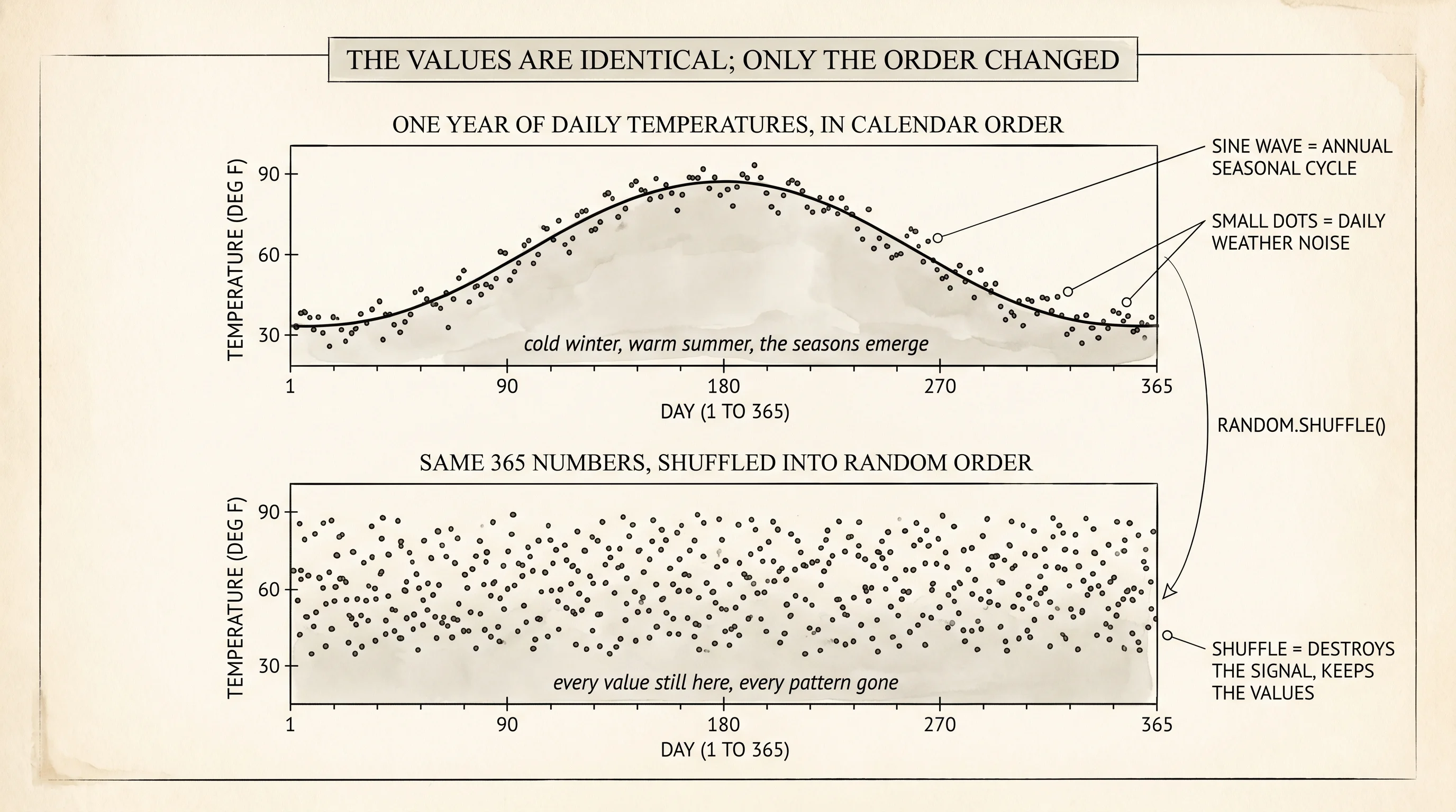
The cleanest way to feel this is one year of weather. Imagine a thermometer in the backyard taking one reading per day for 365 days. The reading climbs from January through July and falls back through December — a slow seasonal curve — with a few degrees of daily wobble on top. Plot that year in calendar order and the shape is obvious: a sine wave with noise. Shuffle the same 365 numbers into a random order and the same numbers are still there, but the shape is gone. The shuffled list looks like static. Nothing changed about the values themselves. Only the order changed, and the order was carrying everything.

Open weather.py in your venv. The first job is to make a year of synthetic temperatures so the lesson is reproducible. A sine wave handles the seasons; a small Gaussian draw per day handles the noise.

import math
import random
 
 
def generate_weather(n_days, base_temp, seasonal_amplitude, daily_noise, seed):
    rng = random.Random(seed)
    temperatures = []
    for day in range(n_days):
        seasonal = seasonal_amplitude * math.sin(2.0 * math.pi * day / 365.0)
        wiggle = rng.gauss(0.0, daily_noise)
        temperatures.append(base_temp + seasonal + wiggle)
    return temperatures
 
 
ordered = generate_weather(365, base_temp=60.0, seasonal_amplitude=25.0, daily_noise=4.0, seed=7)

Print the first 10 days and the middle 10 days to confirm the seasonal arc is real.

print("first 10 days:", [round(t, 1) for t in ordered[:10]])
print("days 180-189:", [round(t, 1) for t in ordered[180:190]])

first 10 days: [60.7, 60.0, 64.2, 61.1, 62.7, 61.7, 64.0, 65.5, 65.1, 66.0]
days 180-189: [85.0, 85.4, 84.0, 85.1, 84.4, 85.5, 84.6, 84.6, 81.5, 79.9]

January is in the low 60s, July is in the mid 80s, the sine wave is doing its job. Now the predictor problem. Each morning you wake up and have to guess today's high. You have all the past days in a notebook. Three guesses are on the table.

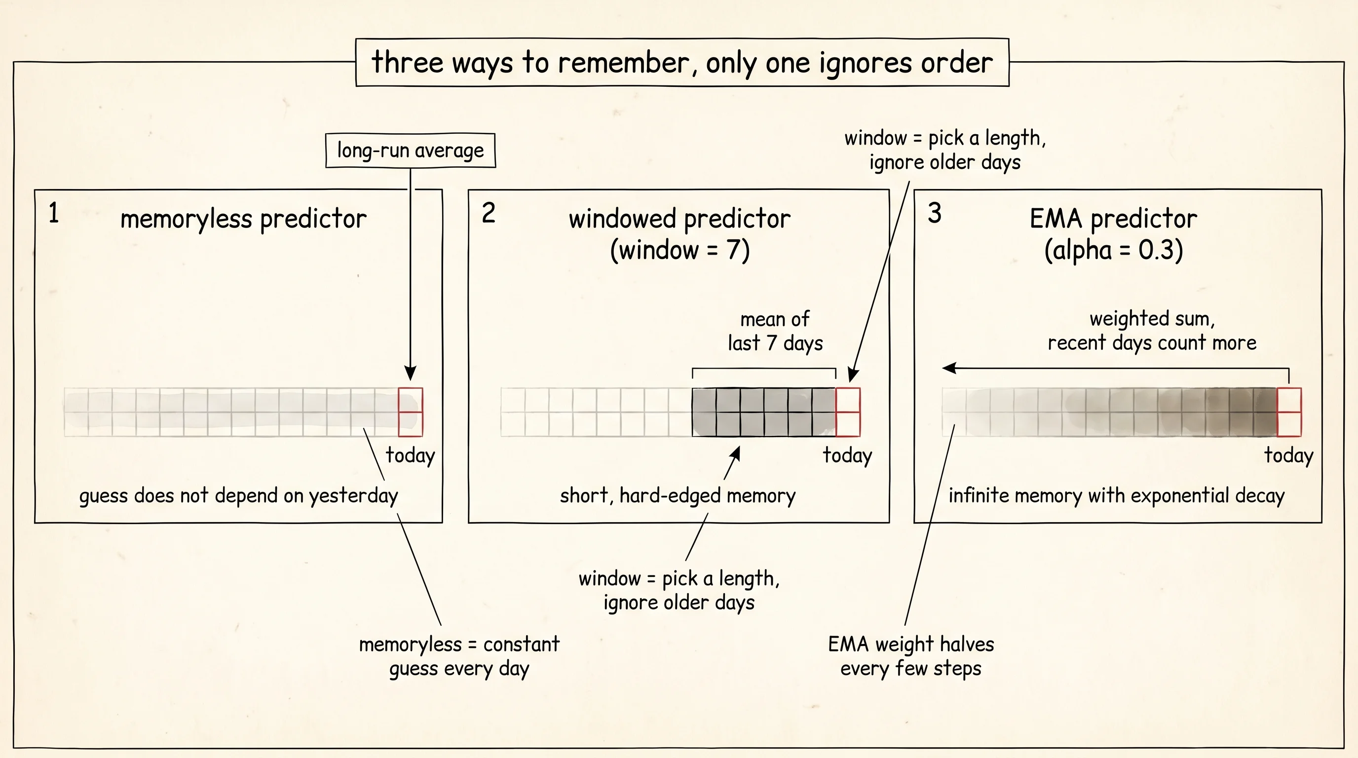
The first guess is the dumb one. Ignore the notebook. Just guess the long-run average. We will call this memoryless because it does not look at order at all. Day 0 has no history, so it gets a free pass. Every later day gets the running mean of all the days before it.

def predict_memoryless(data):
    predictions = [data[0]]
    running_sum = data[0]
    for t in range(1, len(data)):
        predictions.append(running_sum / t)
        running_sum += data[t]
    return predictions

The memoryless predictor will be wrong by a lot in January (it guesses 70-something when the real day is 60) and wrong by a lot in July (it guesses 70-something when the real day is 85). Across the whole year the errors average out, but on any single day the guess is bad.

The second guess uses a fixed window. Average the last 7 days and call it tomorrow. A short memory. If yesterday was 84 and the day before was 83, today is probably also in the low 80s.

def predict_windowed(data, window):
    predictions = [data[0]]
    for t in range(1, len(data)):
        start = max(0, t - window)
        history = data[start:t]
        predictions.append(sum(history) / len(history))
    return predictions

The third guess uses an exponential moving average. The EMA is what you get when you say "yesterday counts most, the day before counts a little less, the day before that counts even less, and so on, with the weight halving every few steps." It is a single rolling number that quietly remembers everything but pays the most attention to the recent past.

def predict_ema(data, alpha):
    predictions = [data[0]]
    ema = data[0]
    for t in range(1, len(data)):
        predictions.append(ema)
        ema = alpha * data[t] + (1.0 - alpha) * ema
    return predictions

Read that loop carefully. The EMA at day t is alpha * today + (1 - alpha) * yesterday's EMA. Set alpha to 1.0 and the EMA forgets everything except today. Set alpha to 0.0 and the EMA never updates. Set alpha to 0.3, and yesterday counts 30 percent and the entire past counts 70 percent. Every older day's contribution shrinks by a factor of 0.7 for every step into the past. After 20 days an old reading is contributing about 1 percent. The memory is long but it fades.

To compare the three, score each one with mean squared error — the same MSE from a few lessons ago. Take the predicted value, subtract the actual value, square it, average over the year.

def evaluate(predictions, actuals):
    total = 0.0
    for predicted, actual in zip(predictions, actuals):
        difference = predicted - actual
        total += difference * difference
    return total / len(actuals)

Now the trick that gives the lesson its name. Generate the year, score every predictor on the year in order, then shuffle the same 365 numbers into random order and score every predictor again. Same values, different order. If order really is the data, the shuffled scores should be much worse for the predictors that lean on order.

def shuffle_days(data, seed):
    rng = random.Random(seed)
    shuffled = list(data)
    rng.shuffle(shuffled)
    return shuffled
 
 
ordered = generate_weather(365, base_temp=60.0, seasonal_amplitude=25.0, daily_noise=4.0, seed=7)
shuffled = shuffle_days(ordered, seed=11)
 
for name, days in [("ordered", ordered), ("shuffled", shuffled)]:
    print(f"\n{name} days:")
    print(f"  memoryless              MSE = {evaluate(predict_memoryless(days), days):8.3f}")
    print(f"  windowed (last 7 days)  MSE = {evaluate(predict_windowed(days, 7), days):8.3f}")
    print(f"  EMA (alpha=0.3)         MSE = {evaluate(predict_ema(days, 0.3), days):8.3f}")

Run it.

ordered days:
  memoryless              MSE =  332.011
  windowed (last 7 days)  MSE =   21.028
  EMA (alpha=0.3)         MSE =   21.663
 
shuffled days:
  memoryless              MSE =  336.023
  windowed (last 7 days)  MSE =  391.572
  EMA (alpha=0.3)         MSE =  400.608

Read the table once across, once down. On the ordered year, the windowed predictor scores 21 and the memoryless predictor scores 332 — the windowed is more than 15 times better. The EMA is right next to the windowed at 22, doing the same job a different way. On the shuffled year, the windowed and EMA collapse to 391 and 400. The memoryless predictor barely moved, from 332 to 336, because it never used order in the first place. Same 365 numbers in both runs. The only difference is which day sat next to which day, and that single difference moved the windowed predictor from "wrong by 5 degrees" to "wrong by 20 degrees."

A small question. The memoryless number went from 332 to 336 on the shuffled run. Why did it move at all if the predictor ignores order?

Because the memoryless predictor uses the running mean of the past, and the running mean walks through the days one at a time. After 30 ordered days the mean is close to the January average, and the predictor's January guess is close to right. After 30 shuffled days the mean is closer to the year-round average of 60, which is wrong for whichever month the random first 30 happened to land in. The shape of the running mean depends on the order it sees the values in. The predictor pretends not to care about order, but the running mean leaks a tiny dose of order through the back door. The clean way to make a truly memoryless predictor is to take the mean of the whole year up front. The slightly leaky way is the one above. Both are still bad on a year of weather. Bad in roughly the same way before and after the shuffle, which is the only point that matters here.

The full project at projects/22-weather-predictor/main.py has a few more touches: it prints a small ASCII strip of the year so you can see the seasonal curve before and after the shuffle, and it prints a delta column showing exactly how much each predictor degraded. Run it once and watch the windowed and EMA scores fall off a cliff while the memoryless one shrugs.

You can predict the next day with a window. Real sequences are not all the same shape. A sentence has 4 words or 40 words. A song has 30 seconds or 6 minutes. A window of size 7 cannot stretch to fit a whole novel and cannot shrink to fit a single phrase. The next move is a network that reads one item, remembers what it just saw, and then reads the next item — a window of size 1 with a memory that grows on its own.