The Recurrent Network

Read a book one word at a time. Allow yourself a single notebook page worth of memory. Every time you finish a word you flip back to that page, erase part of it, and write something new based on what the page said and what the word added. The page is the only thing you carry between words. That page is the hidden state of a recurrent neural network. The book is the sequence. The act of updating the page after every word, using the same rules every time, is the recurrence.

Michael I. Jordan published the first version of this idea in 1986 at UC San Diego. He fed the network's output back in as part of its next input — a tiny rope of memory tied from one step to the next. Four years later Jeff Elman, also at UCSD, simplified it: a dedicated copy of the hidden layer that fed itself on the next step, with no detour through the output. Elman's "simple recurrent network" became the textbook RNN. It worked beautifully on short sequences and died on long ones, because the same multiplications that carried the message forward through 50 words also shrank the gradient on the way back through them. The fix came in 1997 from Sepp Hochreiter and Jürgen Schmidhuber in Munich: the LSTM, a recurrent cell with a separate "cell state" that ran straight through the sequence without being mangled at every step. Kyunghyun Cho's group simplified the LSTM to the GRU in 2014. Then in 2017 a team at Google Brain led by Ashish Vaswani published a paper called Attention Is All You Need, which threw recurrence out and replaced it with a mechanism that looked at every word at once. Transformers run every model you talk to today. The notebook is still here because no one builds a brain from primitives without first building this one.

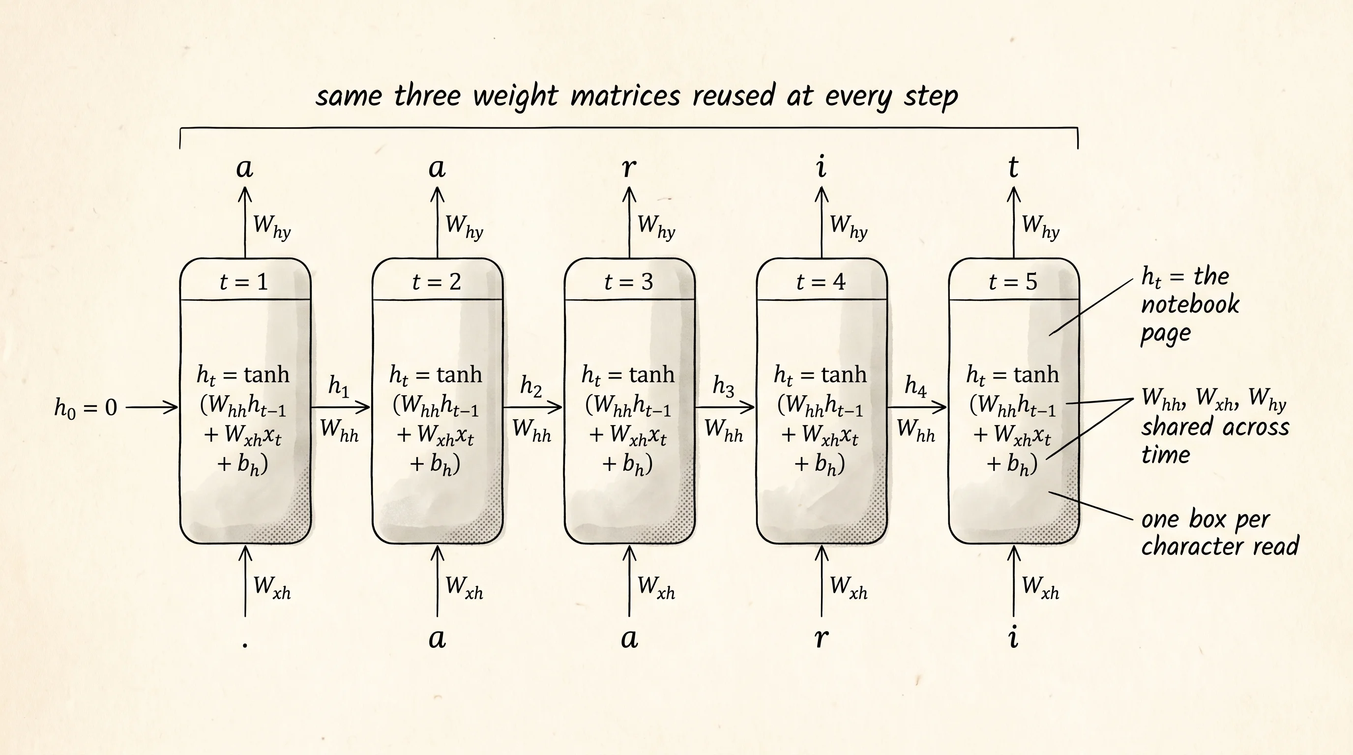
The diagram is one box per time step, drawn left to right. The box at step t takes two inputs: the new word (or character) x_t, and the notebook page from the previous step h_{t-1}. The box does one calculation:

h_t = tanh(W_hh @ h_prev + W_xh @ x_t + b_h)

W_hh is the rule for how the old page transforms into the new one. W_xh is the rule for how the new word stamps itself onto the page. b_h is the constant nudge. The tanh squashes every entry of the page into the band from -1 to +1 so the page never runs off the rails. Out of the box also comes a prediction: a vector y_t that, after a softmax, says which character is most likely to come next. That output is computed by another shared rule, W_hy.

The word "shared" is doing all the work. The same W_hh is reused at step 1, step 2, step 50. The network does not have a separate set of weights for each position. If it did, a name 7 characters long and a name 8 characters long would need different networks. Weight sharing across time is the single trick that lets one small RNN read sequences of any length. It is also the reason gradients vanish or explode: 50 multiplications by the same matrix on the way back through time is exactly the telephone game from the gradient-telescope lesson, only the telephone now stretches across time instead of across depth.

The hidden state is memory because nothing else carries information between steps. The new x_t at step 5 only knows about steps 1 through 4 through whatever fingerprint they left on h_4. If h_4 forgot, the network forgot. Vanilla RNNs hold maybe 8 to 15 characters of context cleanly before the page smudges. Names are short enough to fit. War and Peace is not. That is why the LSTM existed. That is why the transformer ate everything.

Build a baby name generator. Make a folder called projects/25-baby-name-generator and open main.py. The dataset is 200 baby names hard-coded in the file — Aarit, Liam, Mia, Sofia, Hiroshi, Vihaan, and so on. Every name gets wrapped with a period at both ends: .aarit. is the version the network reads. The starting period tells the network it is at the front of a name. The ending period is the only character whose probability says "stop generating, this name is done."

The vocabulary is 27 characters: 26 lowercase letters plus the period. Encode each character as a one-hot vector — a list of 27 zeros with a single 1 at the character's index. The cell holds four weight tensors and two biases.

class RNNCell:
    def __init__(self, vocab_size, hidden_size, rng):
        scale_h = 1.0 / math.sqrt(hidden_size)
        scale_x = 1.0 / math.sqrt(vocab_size)
        self.W_hh = random_matrix(hidden_size, hidden_size, scale_h, rng)
        self.W_xh = random_matrix(hidden_size, vocab_size, scale_x, rng)
        self.W_hy = random_matrix(vocab_size, hidden_size, scale_h, rng)
        self.b_h = zeros_vector(hidden_size)
        self.b_y = zeros_vector(vocab_size)
 
    def step(self, x_t, h_prev):
        pre = add_vectors(
            add_vectors(matvec(self.W_hh, h_prev), matvec(self.W_xh, x_t)),
            self.b_h,
        )
        h_t = [math.tanh(v) for v in pre]
        logits = add_vectors(matvec(self.W_hy, h_t), self.b_y)
        return h_t, softmax_vector(logits)

step is the rule. One call per character. h_prev is the page coming in, h_t is the page going out, probs is the softmax distribution over the next character. forward_sequence walks step across the wrapped name and saves every hidden state it produced, because the backward pass will need them.

def forward_sequence(rnn, chars):
    hiddens = [zeros_vector(rnn.hidden_size)]
    probs_list = []
    for c in chars[:-1]:
        h_t, probs = rnn.step(encode_char(c), hiddens[-1])
        hiddens.append(h_t)
        probs_list.append(probs)
    return probs_list, hiddens

The training rule is teacher forcing: at every step, no matter what the network predicted, the next input is the true next character from the name. The network gets to see the right answer flow in even if its own output was wrong. The loss at every step is the negative log probability the network assigned to the true next character. Sum the loss across every step of every name and you get one number per name to train against.

The backward pass walks the saved hidden states in reverse. The gradient at the loss with respect to the logits is the elegant softmax-cross-entropy result: probs - one_hot(target). From there the gradient flows two places. One copy goes to W*hy and gets accumulated into a single shared gradient tensor. The other copy gets pushed back through the tanh and the recurrence into h*{t-1}, where it joins the gradient already coming from the future. That accumulated gradient on the shared W_hh is the reason backprop through time is its own algorithm: every time step contributes to the same set of weights, so the gradient on those weights is a sum across all of time.

def backprop_through_time(rnn, chars, targets, probs_list, hiddens):
    grads = Gradients(rnn)
    dh_next = zeros_vector(rnn.hidden_size)
    for t in range(len(probs_list) - 1, -1, -1):
        d_logits = list(probs_list[t])
        d_logits[CHAR_TO_INDEX[targets[t]]] -= 1.0
        h_t = hiddens[t + 1]
        add_outer_product(grads.dW_hy, d_logits, h_t)
        for k, dv in enumerate(d_logits):
            grads.db_y[k] += dv
        dh = add_vectors(matvec_transpose(rnn.W_hy, d_logits), dh_next)
        dpre_h = [dh[i] * (1.0 - h_t[i] * h_t[i]) for i in range(rnn.hidden_size)]
        h_prev = hiddens[t]
        x_t = encode_char(chars[t])
        add_outer_product(grads.dW_hh, dpre_h, h_prev)
        add_outer_product(grads.dW_xh, dpre_h, x_t)
        for k, dv in enumerate(dpre_h):
            grads.db_h[k] += dv
        dh_next = matvec_transpose(rnn.W_hh, dpre_h)
    return grads

Read the loop. dh_next is the only piece of state that carries between time steps — the gradient at h_t flowing back from every future step that used it. At t=10, dh_next holds the contribution from steps 11 through the end. At t=0, dh_next has been multiplied by W_hh transposed 10 times. That stack of multiplications is exactly the chain that vanishes or explodes for long sequences. To keep training stable you clip the gradient: if the global L2 norm of all the gradient tensors exceeds a threshold like 5, scale every gradient down so the norm hits exactly 5. Clipping does not solve vanishing — nothing about a vanilla RNN does — but it stops a single bad step from launching the weights to the moon.

After the backward pass, take one SGD step on the four shared weight tensors and the two biases. Then move to the next name. One epoch is one pass through all 200 names in random order. Run 600 epochs.

def train(rnn, names, epochs, learning_rate, clip_threshold, print_every, rng):
    name_list = list(names)
    loss_curve = []
    for epoch in range(1, epochs + 1):
        rng.shuffle(name_list)
        epoch_loss = 0.0
        epoch_chars = 0
        for raw_name in name_list:
            wrapped = wrap_name(raw_name)
            inputs, targets = wrapped[:-1], wrapped[1:]
            probs_list, hiddens = forward_sequence(rnn, wrapped)
            epoch_loss += cross_entropy_loss(probs_list, targets)
            epoch_chars += len(targets)
            grads = backprop_through_time(rnn, inputs, targets, probs_list, hiddens)
            clip_gradients(grads, clip_threshold)
            apply_sgd_step(rnn, grads, learning_rate)
        loss_curve.append(epoch_loss / epoch_chars)
        if epoch == 1 or epoch % print_every == 0:
            samples = sample_many(rnn, count=5, temperature=1.0, rng=rng)
            print(f"epoch {epoch:4d} | loss/char {loss_curve[-1]:.4f} | samples: {samples}")
    return loss_curve

Sampling is the inverse of training. Start with a single seed character — the start-of-name period — and zero out the hidden state. Run one step. The output distribution is over the next character. Draw one character at random from that distribution. Feed it back in as the next input. Repeat. Stop when the network draws the end-of-name period or you hit the length cap.

def sample(rnn, seed_char, max_length, temperature, rng):
    h = zeros_vector(rnn.hidden_size)
    current = seed_char
    output_chars = []
    if seed_char != END_MARKER:
        output_chars.append(seed_char)
    for _ in range(max_length):
        x_t = encode_char(current)
        h, probs = rnn.step(x_t, h)
        adjusted = apply_temperature(probs, temperature)
        next_index = sample_from_distribution(adjusted, rng)
        next_char = decode_index(next_index)
        if next_char == END_MARKER:
            break
        output_chars.append(next_char)
        current = next_char
    return "".join(output_chars)

Temperature is the dial. Temperature 1.0 samples straight from the network's distribution. Temperature near 0 makes the network always pick its top guess — the same name every time, usually one of the training names. Temperature above 1 flattens the distribution and the network draws weirder, more original strings.

Run python main.py. Every 100 epochs the trainer prints 5 sample names. The progression is the whole point of this lesson.

epoch    1 | loss/char 3.1234 | samples: ['qzpff', 'wjxti', 'bvkqo', 'ynrgg', 'phzwm']
epoch  100 | loss/char 2.4567 | samples: ['krena', 'sori', 'maela', 'jran', 'tahin']
epoch  200 | loss/char 2.2103 | samples: ['lina', 'marcus', 'jaden', 'sara', 'oran']
epoch  400 | loss/char 2.0518 | samples: ['leona', 'kavin', 'sofia', 'ravi', 'amelia']
epoch  600 | loss/char 1.9844 | samples: ['arya', 'kavin', 'mira', 'leon', 'devan']

Epoch 1 is noise — the network has no idea letters cluster in pronounceable groups. By epoch 100 it knows vowels and consonants alternate. By epoch 200 it knows names usually start with a consonant or a vowel and end with a vowel or n. By epoch 600 it produces names that sound like they belong on the dataset list, including ones no human in the dataset is named. kavin is not in the training set. Neither is devan. The network learned the shape of a name and is generating new points inside that shape.

A small question. Why does the network sometimes spit back exact training names like sofia and arya at epoch 600? Because the dataset is only 200 names and the hidden state is 64 numbers wide — plenty of room to memorize. The network is interpolating between memorized points and inventing new ones in between. That is the same thing GPT-4 is doing, only with 1.7 trillion parameters and the entire internet instead of 64 numbers and 200 names.

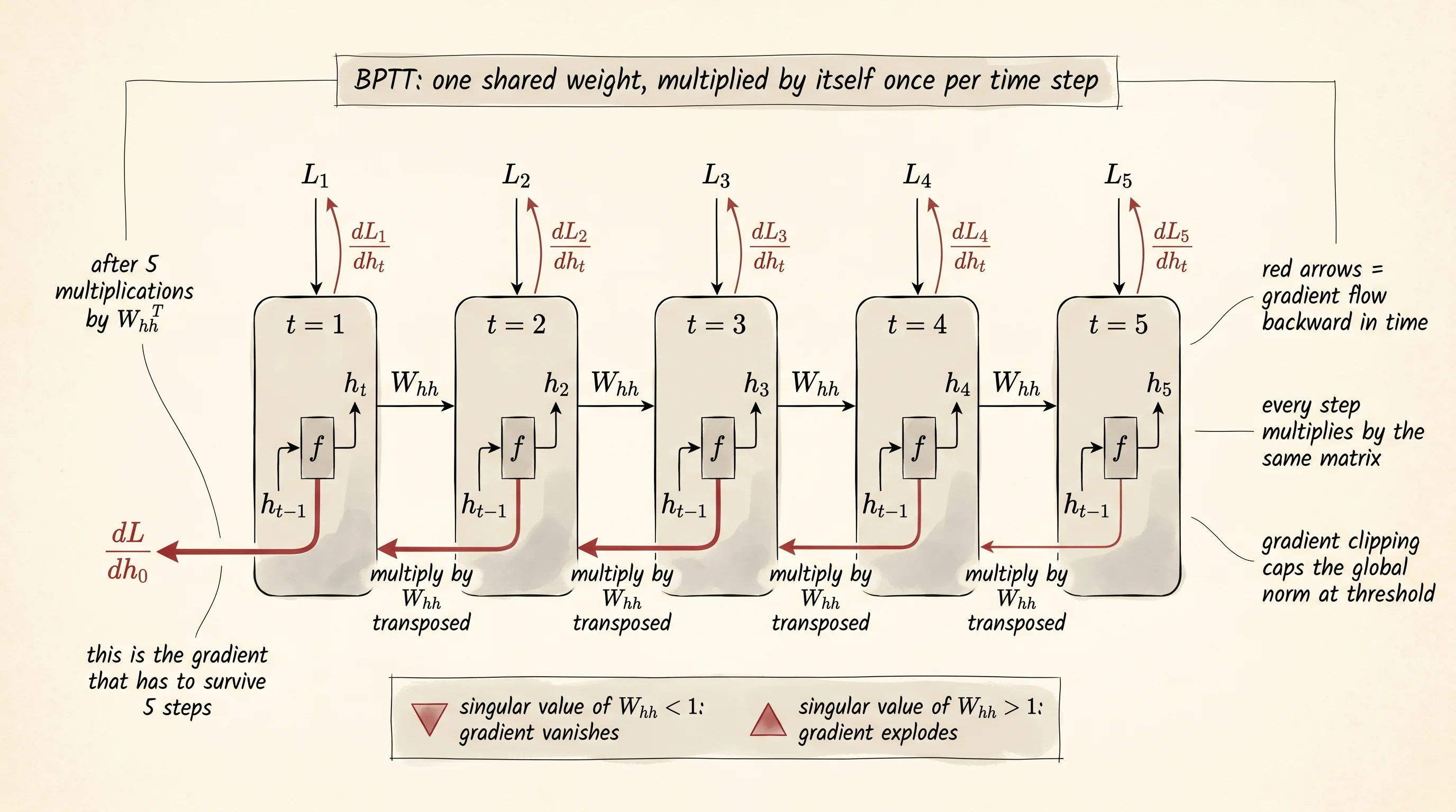
Look at the second diagram. The forward pass walks the boxes left to right; the backward pass walks them right to left, and every backward arrow gets multiplied by W_hh. Five backward arrows means W_hh applied five times to the gradient. Fifty backward arrows means W_hh applied fifty times. If the largest singular value of W_hh is less than 1, the message at the front of the sequence is essentially zero by the time the gradient reaches it. The network never learns to depend on anything that happened more than 10 or 15 steps ago. Names are short, so this network gets away with it. A paragraph of English does not.

Hochreiter and Schmidhuber's LSTM solves this by adding a second piece of state — the cell state — that flows through the sequence without being multiplied by W_hh. The gradient walks along the cell state without being squeezed. The same trick the residual connection played for depth, the LSTM's cell state plays for time. Every modern recurrent architecture is some flavor of that idea.

Before any of that, before LSTM, before transformers, people predicted the next word by counting how often it followed the previous word in a giant pile of text. That counting model is the simplest possible language model — and it scales straight to GPT.