N-Gram Language Models

A medieval scribe is copying a long manuscript by candlelight. He has been at it for hours and his eyes are blurry. He cannot remember a whole sentence. He can barely remember the last letter he wrote. Every time his quill comes back to the page he glances at the last letter, asks himself "what letter usually comes after this one?", and writes the next one. No grammar. No meaning. Just the habit of which letters tend to follow which other letters. That scribe is the simplest language model anyone has ever built, and the brain you are about to write thinks exactly the way he does.

The first person to do this on purpose was a Russian mathematician named Andrey Markov in 1906. Markov sat down with a copy of Pushkin's novel Eugene Onegin and counted, by hand, how often a vowel followed a vowel and how often a vowel followed a consonant for the first 20,000 letters of the book. He was trying to settle an argument: a colleague claimed that statistics only worked on independent events, like coin flips, and could not say anything about events where one outcome influenced the next. Markov's tally proved his colleague wrong. The letters in Russian poetry were not independent. The letter you saw last told you something real about the letter that was coming. He published the table and named the idea after himself. A Markov chain is a system where the next state depends only on the current state, nothing further back. Forty-two years later, in 1948, Claude Shannon picked up Markov's idea and ran it on English in the founding paper of information theory. Shannon counted single-letter, two-letter, and three-letter frequencies in a stack of English texts and showed that the longer the context you remembered, the more your generated text started to look like English. The mental model in this lesson is exactly the mental model behind GPT. Replace the count table with a transformer, replace the characters with word pieces, and you have ChatGPT.

The brain has 3 jobs and they all use the same idea: counting. First, read a piece of text and tally up how often each letter follows each other letter. Second, turn those counts into probabilities so they add up to 1 for every starting letter. Third, generate new text by rolling a weighted die against those probabilities, one letter at a time. The full model is a dictionary that maps a context (the last 1 or 2 characters) to a Counter of which characters showed up next.

from collections import Counter
 
def build_ngram_counts(text, n):
    table = {}
    context_size = n - 1
    for i in range(len(text) - context_size):
        context = text[i : i + context_size]
        next_char = text[i + context_size]
        if context not in table:
            table[context] = Counter()
        table[context][next_char] += 1
    return table

A bigram model has n = 2, so the context is the last 1 character. A trigram model has n = 3, so the context is the last 2 characters. Walk through this on a tiny string by hand and the loop becomes obvious.

counts = build_ngram_counts("the cat sat", n=2)
print(counts["t"])
print(counts["h"])

The output:

Counter({'h': 1, ' ': 1})
Counter({'e': 1})

After t the model has seen h once (in the) and a space once (in cat and sat ends with t — actually only cat here). After h it has seen e once. The Counter is the brain's memory of "after this letter, here is what came next, and how often."

Counts are not probabilities. To sample, you need numbers that add to 1. Divide each count by the total for that context.

def normalize_counts(counts):
    probs = {}
    for context, counter in counts.items():
        total = sum(counter.values())
        probs[context] = {char: count / total for char, count in counter.items()}
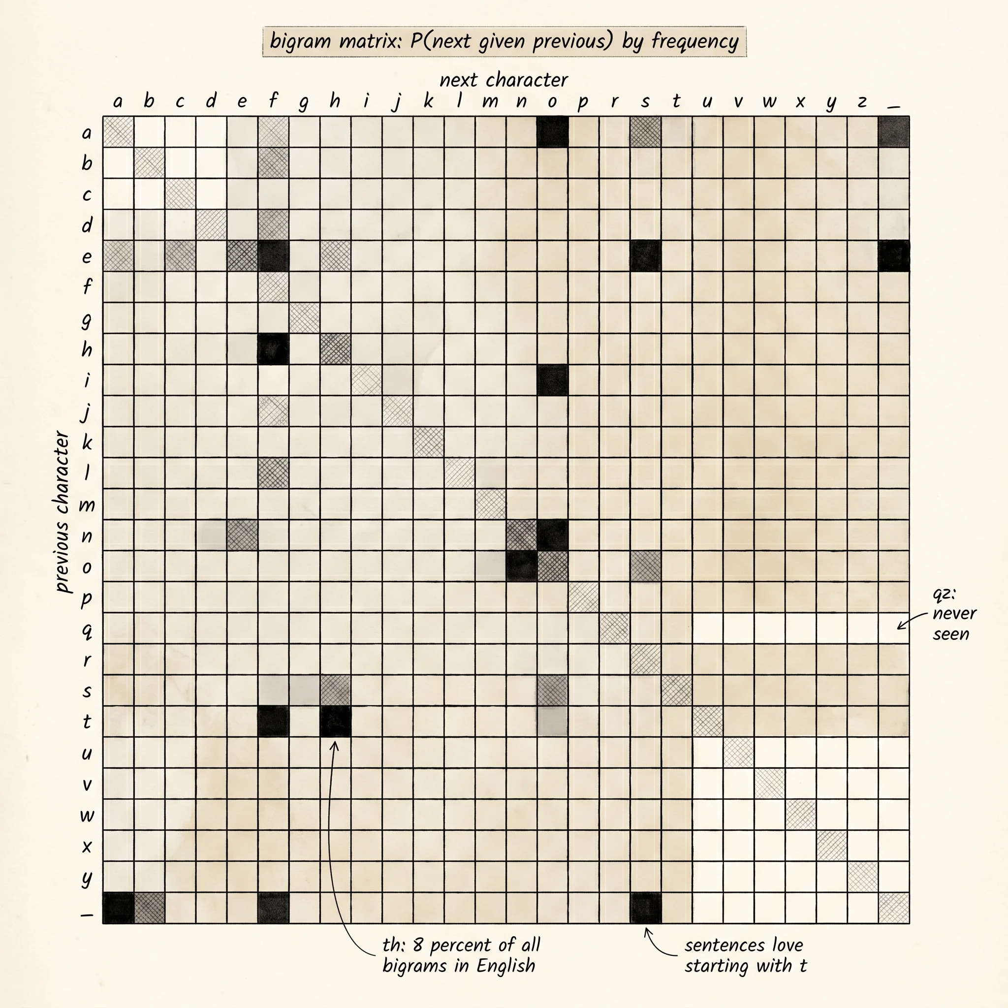
    return probs

The probability table for the context t becomes {'h': 0.5, ' ': 0.5}. Half the time t was followed by h, half the time by a space. For a real corpus the brain ends up with a much sharper picture: in a children's storybook, t is followed by h close to half the time, by a space about a quarter, and by everything else in small slivers. The brain has learned a habit it never had to be told.

Sampling from a probability table is the same trick from the softmax lesson. Roll a uniform number between 0 and 1. Walk down the entries adding their probabilities to a running total. The first entry whose running total passes the roll is the pick.

import random
 
def sample_next(distribution):
    threshold = random.random()
    running = 0.0
    last_char = ""
    for char, probability in distribution.items():
        running += probability
        last_char = char
        if threshold < running:
            return char
    return last_char

If distribution is {'h': 0.5, ' ': 0.5} and the roll is 0.3, the running total reaches 0.5 on the first entry, 0.3 is below 0.5, so the function returns 'h'. If the roll is 0.7 the first entry pushes running to 0.5, that is below 0.7, the second entry pushes running to 1.0, that is above 0.7, so the function returns the space. The roll picks h 50% of the time and a space 50% of the time.

Stack the pieces and the model can write. Start with a seed. Look up the last 1 or 2 characters in the probability table. Sample the next character. Append it. Repeat. This is autoregressive generation — each step's input is the previous step's output. Real GPT-class models do the same dance with billions of parameters where the count table sits.

def generate(probs, seed, length, n):
    context_size = n - 1
    output = list(seed)
    known = list(probs.keys())
    for _ in range(length):
        context = "".join(output[-context_size:])
        if context not in probs:
            context = random.choice(known)
        next_char = sample_next(probs[context])
        output.append(next_char)
    return "".join(output)

The fallback in the middle handles the case where the chain wanders into a context the model never saw. The bigram model never sees an unknown context — there are only so many single characters. The trigram model can. If the training text never contained qx and the chain happens to produce q followed by x, the lookup misses. The fallback grabs any context the model knows and keeps going. A real model would smooth this with a more careful backoff scheme. This version simply re-seeds.

The whole project lives in projects/30-text-statistics-engine/main.py. The training corpus is a short fairy tale about a miller and his three sons. Build the bigram model, build the trigram model, and ask each one to write 200 characters of new story.

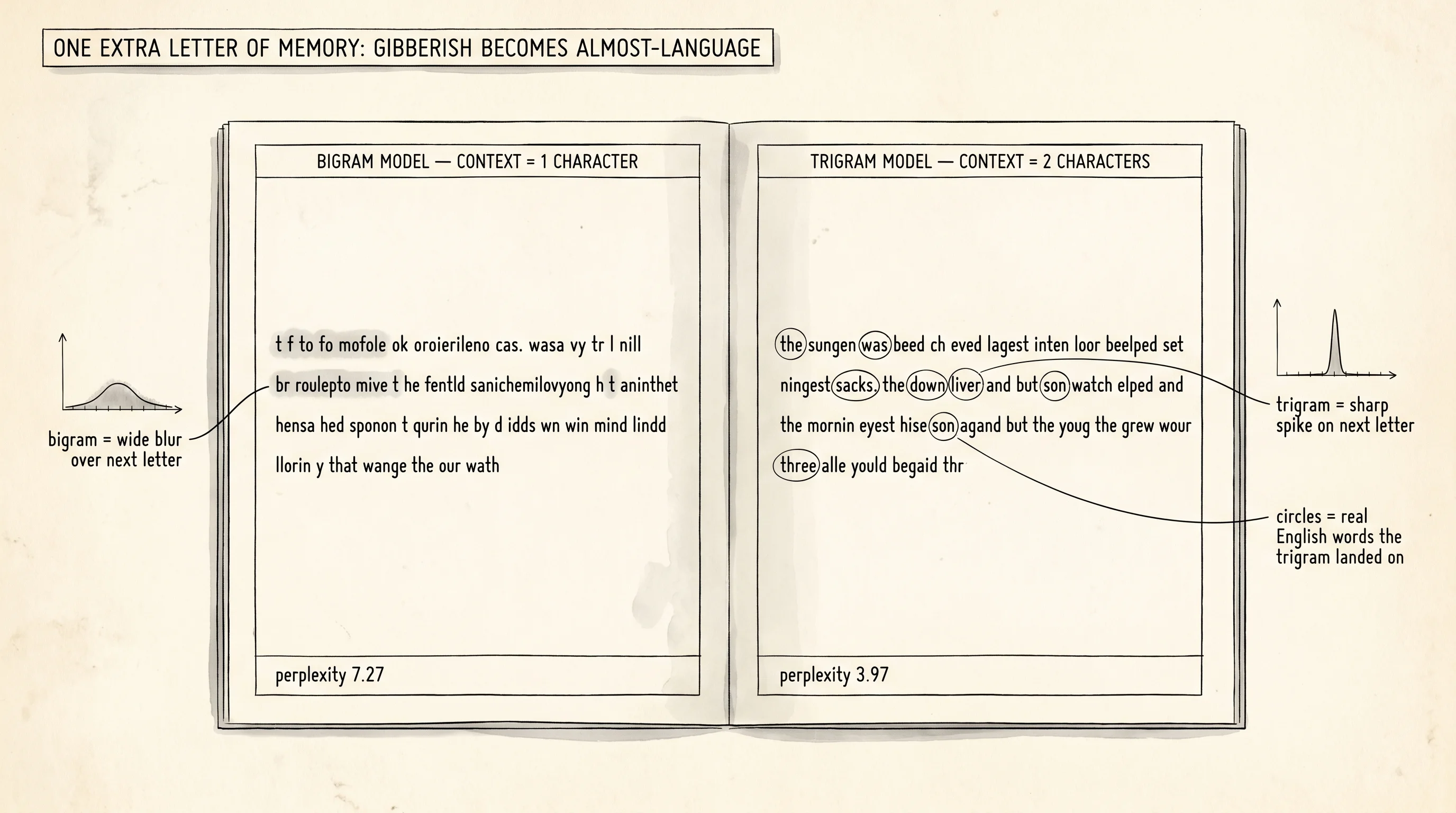
--- 200 characters from bigram model ---
t f to fo mofole ok oroierileno cas. wasa vy tr l nill br roulepto mive t he fentld sanichemilovyong
h t aninthethensa hed sponon t qurin he by d idds wn win mind lindd llorin y that wange the our wath
 
--- 200 characters from trigram model ---
the sungen was beed ch eved lagest inten loor beelped set ningest sacks. the down liver and but son
watch elped and the mornin eyest hise son agand but the youg the grew wour three alle yould begaid thr

Read the bigram output. It is gibberish. There are no real words. The brain that only remembers the last single letter has too little context to ever land on a real word longer than 2 or 3 letters. It does pick up a few real fragments — the, wasa, mind — but only because those letter pairs are common everywhere. Read the trigram output. The change is dramatic. the, sacks., was, son, down, liver, but, three are real words. sungen, lagest, inten, mornin are not real words but they look like real words. They have the shape and texture of English. The brain that remembers 2 characters instead of 1 has crossed the line from random letters to almost-language.

A small question. Why does adding 1 character of memory make such a huge difference? After all, the trigram model only knows 1 more character than the bigram model. The answer is in how sharp the probability table becomes. After the single letter h, the bigram model's distribution is spread across many possible next letters because h shows up in the, he, which, house, every English word with an h. After the 2 letters th, the trigram model's distribution collapses almost entirely onto e — the is so much more common than tha, tho, thi that the model picks e about 80% of the time. One extra character of memory shrinks the next-character distribution from a wide blur into a sharp spike. Sharp spikes produce real word fragments. Wide blurs produce noise.

To put a number on how much better the trigram model is, measure perplexity. Perplexity is the average number of choices the model effectively faces at each step. A perplexity of 27 means the model is as confused as if it had to pick uniformly between 27 letters at each step — useless. A perplexity of 4 means the model is as sure as if it only had 4 plausible next letters at each step — sharp. Compute it as the exponential of the average negative log probability the model assigned to a held-out chunk of the corpus.

import math
 
def perplexity(probs, test_text, n, floor=1e-3):
    context_size = n - 1
    total_log_prob = 0.0
    steps = 0
    for i in range(len(test_text) - context_size):
        context = test_text[i : i + context_size]
        next_char = test_text[i + context_size]
        if context in probs and next_char in probs[context]:
            probability = probs[context][next_char]
        else:
            probability = floor
        total_log_prob += math.log(probability)
        steps += 1
    return math.exp(-total_log_prob / steps)

Hold out the last 15% of the corpus from training. Train on the first 85%. Score the held-out text with both models.

bigram perplexity:  7.274
trigram perplexity: 3.970

The trigram is roughly half as confused per character. The bigram is rolling a 7-sided die at every position, the trigram is rolling a 4-sided die. That is the entire difference between the two systems on this corpus. More context shrinks the die.

Shannon ran this same experiment on English text in 1948 and reached the same conclusion: more context, lower perplexity, more readable output. He went on to estimate that English text has about 1 bit of entropy per character once you condition on a long enough history, which means a perfect model would have a perplexity of 2. Modern transformer language models are within striking distance of that floor. Markov, Shannon, GPT — the same idea, applied with more compute and more memory each round.

The brain you just built has 1 fatal limit. It can only remember contexts it has literally seen during training. Show the trigram model the context qx and it has nothing — no answer, no guess, no notion that qx is similar to qu or xy in any way. Every context is a separate row of the table with no relationship to any other row. The next lesson teaches the network how to give similar contexts similar predictions even when the exact context never appeared in training, which is the trick that takes language models from memory to generalization.