Embeddings as Lookup Tables
The trigram brain at the end of the last lesson had one fatal habit. Every context was a separate row in a giant table, and the rows did not know each other. The row for qu and the row for qa sat in different cells of the cabinet with no wire between them, even though anyone who reads English knows the two contexts behave almost the same way. The brain could memorize. The brain could not generalize. The fix is to throw out the cabinet of strings and replace every word with a short list of numbers — a vector — that the network gets to pick for itself during training. The first time anyone did this on purpose was Yoshua Bengio's lab at the University of Montreal in 2003.
Bengio and his graduate students Réjean Ducharme, Pascal Vincent, and Christian Jauvin had been staring at a wall called the curse of dimensionality. A 100,000-word vocabulary needs a count table with 100,000 to the third power cells to model trigrams, which is a quadrillion. Smoothing tricks helped, but the system never learned that "the cat is walking in the bedroom" tells you anything about "a dog was running in a room." The two sentences shared no n-grams. They shared meaning. Bengio's team published A Neural Probabilistic Language Model and proposed something the field had been circling since the 1980s: hand each word a short vector of real numbers, train those vectors as part of the network, and let the gradient pull similar-meaning words near each other in the vector space. Ten years later, in 2013, a Czech researcher at Google named Tomas Mikolov took the idea to its logical end with Word2Vec and published the famous result that king minus man plus woman lands almost exactly on queen. The vectors had learned analogy. The same year Jeffrey Pennington, Richard Socher, and Christopher Manning at Stanford released GloVe, which extracted similar vectors by factoring a co-occurrence matrix instead of running a network. The next lesson is GloVe. This lesson is the lookup table.
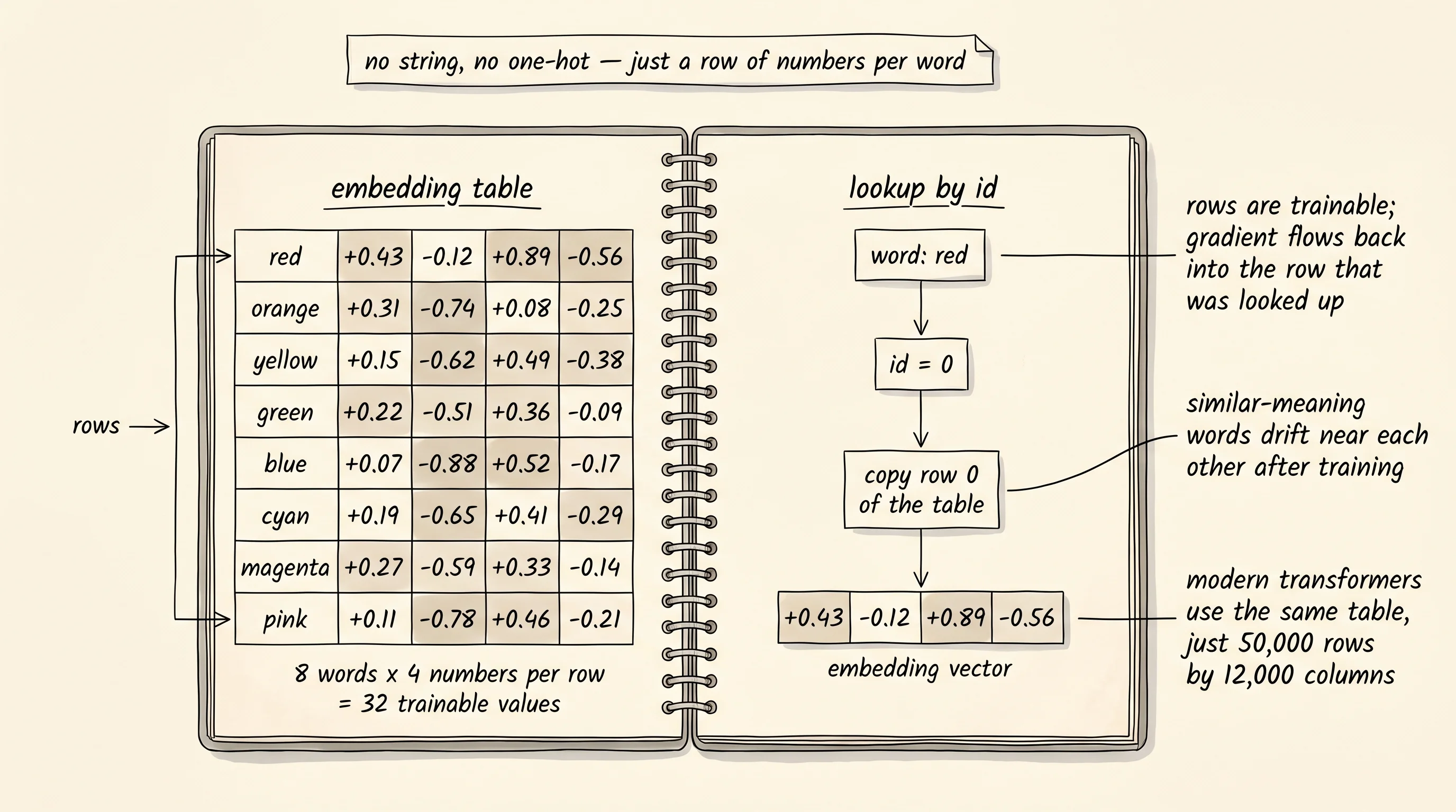
The setup is a notebook with one row per word. Each row is a list of, say, 4 numbers. The notebook starts with random scribbles in every row. To use the notebook, take the integer id of a word and copy out row number id. That copy is the word's embedding. The first thing the network sees is no longer a string, no longer a one-hot vector with a single 1 in a sea of zeros — it is the row of numbers the notebook handed back. Every other layer in the network treats those numbers like any other input. The trick is that the rows themselves are trainable. The gradient that flows back to the input layer does not stop at the embedding lookup. It flows into the row that was looked up and tells the notebook how to nudge those 4 numbers next time.
class EmbeddingTable:
    def __init__(self, vocab_size, embedding_dim):
        scale = 0.5
        self.weights = [
            [random.gauss(0.0, scale) for _ in range(embedding_dim)]
            for _ in range(vocab_size)
        ]
        self.grad = [[0.0] * embedding_dim for _ in range(vocab_size)]

    def lookup(self, index):
        return list(self.weights[index])

    def accumulate_grad(self, index, upstream):
        for d in range(len(upstream)):
            self.grad[index][d] += upstream[d]
Lookup is a list index. There is no math at all in the forward pass — just a copy. The math happens in accumulate_grad, which adds the upstream gradient to the row that was used. Rows that were never looked up at all during a training step get no gradient and do not move. This is the entire mechanical difference between an embedding layer and a normal layer. A linear layer touches every weight on every example. An embedding layer touches only the rows it actually looked up. With a vocabulary of 50,000 words and a batch that mentions 100 words, the embedding layer updates 100 rows and ignores 49,900. That sparsity is why embeddings are cheap even when the vocabulary is huge.
To watch the table earn its rows, give the network a job small enough to reason about. Pick 16 named colors arranged around a wheel — red, red-orange, orange, yellow-orange, yellow, yellow-green, green, blue-green, cyan, sky-blue, blue, blue-violet, violet, magenta, pink, red-pink. Hand each color the integer id of its slot in the list. Build a labeled dataset of color pairs: a pair is harmonious if the two colors sit next to each other on the wheel (analogous, like red and red-orange) or directly across from each other on the wheel (complementary, like red and cyan). A pair is clashing if the two colors are 2 to 5 steps apart on the wheel — far enough to feel wrong, close enough to look muddy. Every color paired with itself is harmonious. The full project is in projects/31-color-harmony-predictor/main.py.
COLOR_NAMES = [
    "red", "red_orange", "orange", "yellow_orange",
    "yellow", "yellow_green", "green", "blue_green",
    "cyan", "sky_blue", "blue", "blue_violet",
    "violet", "magenta", "pink", "red_pink",
]

def harmony_dataset():
    pairs = []
    half = len(COLOR_NAMES) // 2
    for left in range(len(COLOR_NAMES)):
        for right in range(len(COLOR_NAMES)):
            distance = abs(left - right)
            wheel_distance = min(distance, len(COLOR_NAMES) - distance)
            if wheel_distance == 0 or wheel_distance == 1 or wheel_distance == half:
                pairs.append((left, right, 1.0))
            elif 2 <= wheel_distance <= 5:
                pairs.append((left, right, 0.0))
    return pairs
The brain on top of the embedding table is the smallest MLP that can do anything. Look up two colors. Concatenate the two 4-number rows into one 8-number vector. Push that through a hidden layer with 16 ReLU neurons. Push the hidden layer through a single output neuron. Squash the output through a sigmoid to get a probability between 0 and 1. The whole network has 4 sets of trainable numbers: the 16 by 4 embedding table, the 16 by 8 hidden weights, the 1 by 16 output weights, and the biases. About 220 numbers in total. Train with binary cross-entropy and gradient descent. Note one thing: the gradient that lands on the 8-dimensional concatenated input has to be split in half — the first 4 numbers update the left color's row, the last 4 update the right color's row. Every other layer is plain matrix arithmetic from the previous lessons.
def forward_with_cache(self, left_id, right_id):
    left_vec = self.embeddings.lookup(left_id)
    right_vec = self.embeddings.lookup(right_id)
    concat = left_vec + right_vec
    hidden_pre = self.hidden.forward(concat)
    hidden_post = [relu(value) for value in hidden_pre]
    logit = self.output.forward(hidden_post)[0]
    return sigmoid(logit), {
        "concat": concat, "hidden_pre": hidden_pre, "hidden_post": hidden_post,
    }

def backward(self, left_id, right_id, prediction, label, cache):
    d_logit = prediction - label
    d_hidden_post = self.output.backward(cache["hidden_post"], [d_logit])
    d_hidden_pre = [
        d_hidden_post[j] * relu_grad(cache["hidden_pre"][j])
        for j in range(len(d_hidden_post))
    ]
    d_concat = self.hidden.backward(cache["concat"], d_hidden_pre)
    d_left = d_concat[: self.embedding_dim]
    d_right = d_concat[self.embedding_dim :]
    self.embeddings.accumulate_grad(left_id, d_left)
    self.embeddings.accumulate_grad(right_id, d_right)
Train for 200 epochs with a learning rate of 0.1.
--- before training ---
loss = 0.6625  accuracy = 61.46%

epoch   0: running_loss = 0.6945  eval_loss = 0.6264  accuracy = 66.67%
epoch  25: running_loss = 0.1258  eval_loss = 0.0933  accuracy = 96.35%
epoch  50: running_loss = 0.0005  eval_loss = 0.0005  accuracy = 100.00%
epoch 100: running_loss = 0.0002  eval_loss = 0.0002  accuracy = 100.00%
epoch 199: running_loss = 0.0001  eval_loss = 0.0001  accuracy = 100.00%
The network is right on every pair after 50 epochs. A network with 220 numbers learned to score 192 color pairs perfectly. The interesting question is not whether the network learned. The interesting question is what the rows of the embedding table look like now that the gradient has finished pushing them around. Print all 16 rows.
   0 red           -> [-0.605  -1.719  -0.013  +1.242]
   1 red_orange    -> [-1.305  -1.434  +1.350  +0.580]
   2 orange        -> [-0.696  -0.013  +2.696  -0.337]
   3 yellow_orange -> [-0.216  +1.673  +1.556  -1.152]
   4 yellow        -> [+0.948  +1.451  -0.071  -1.953]
   5 yellow_green  -> [+1.007  +1.637  -1.397  -0.551]
   6 green         -> [+0.585  +0.561  -2.578  +0.544]
   7 blue_green    -> [+0.914  -0.953  -1.302  +1.591]
   8 cyan          -> [-0.874  -1.382  +0.051  +2.042]
   9 sky_blue      -> [-1.040  -1.281  +1.347  +0.708]
  10 blue          -> [-0.765  -0.023  +2.156  -0.476]
  11 blue_violet   -> [+0.323  +1.355  +1.592  -1.368]
  12 violet        -> [+0.470  +1.730  -0.285  -1.583]
  13 magenta       -> [+1.183  +1.361  -1.663  -0.773]
  14 pink          -> [+1.263  +0.182  -2.468  +0.586]
  15 red_pink      -> [+0.745  -0.866  -1.197  +1.770]
Numbers do not mean much by themselves. The thing to measure is which rows ended up close together. Cosine similarity is the standard tool: take the dot product of two vectors, divide by the product of their lengths, and you get a number between -1 and 1. Plus 1 means the two vectors point the same direction. Zero means they are perpendicular. Minus 1 means they point opposite directions. Compute the cosine similarity for every pair of color rows and print the table.
                   red red_or orange yellow yellow yellow  green blue_g   cyan
  red            +1.00  +0.74  -0.00  -0.74  -0.95  -0.76  -0.10  +0.57  +0.94
  red_orange     +0.74  +1.00  +0.64  -0.11  -0.72  -0.99  -0.71  -0.11  +0.69
  orange         -0.00  +0.64  +1.00  +0.65  -0.03  -0.63  -0.98  -0.68  +0.01
  yellow_orange  -0.74  -0.11  +0.65  +1.00  +0.65  +0.16  -0.54  -0.90  -0.65
  yellow         -0.95  -0.72  -0.03  +0.65  +1.00  +0.71  +0.07  -0.55  -1.00
  yellow_green   -0.76  -0.99  -0.63  +0.16  +0.71  +1.00  +0.72  +0.05  -0.68
  green          -0.10  -0.71  -0.98  -0.54  +0.07  +0.72  +1.00  +0.63  -0.04
  blue_green     +0.57  -0.11  -0.68  -0.90  -0.55  +0.05  +0.63  +1.00  +0.58
  cyan           +0.94  +0.69  +0.01  -0.65  -1.00  -0.68  -0.04  +0.58  +1.00
Read the row for red. Red points the same way as cyan with a similarity of 0.94. Red points the same way as red-orange with a similarity of 0.74. Red points the opposite direction from yellow with -0.95 and from violet with -0.98. The strongest neighbor of red is cyan. The strongest neighbor of blue is orange. The strongest neighbor of green is pink. Look at the wheel for a moment. Cyan is the complement of red. Orange is the complement of blue. Pink is the complement of green. The network put each color and its complement on the same line through the origin, pointing the same way.
A small question. The lesson promised that similar things end up near each other after training. Red and red-orange are similar — they sit next to each other on the wheel. Their cosine is 0.74. But red and cyan are opposites on the wheel, and their cosine is 0.94. Why did opposites end up closer than neighbors? The label tells the network everything. Both analogous pairs (red with red-orange) and complementary pairs (red with cyan) were labeled harmonious. The network had to put both kinds of partner near each color. The cleanest way to put 2 different partners near a single color is to put both partners together with the color on the same line, and that is exactly what the network did. The "definition" the network wrote for each color is not "this is the visual look of red" — it is "these are the colors red gets along with." Embeddings learn the structure the loss asks for, not the structure a human would have asked for.
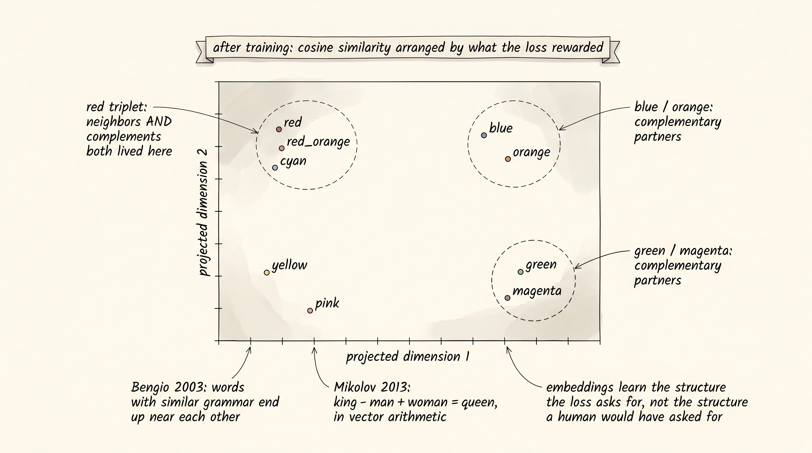
Bengio's team noticed the same effect in their 2003 paper with words. They trained a model to predict the next word in a sentence and then printed the embeddings. Words with similar grammatical roles ended up near each other — Monday near Tuesday, June near July, France near Spain. The network was never told what days or months or countries are. It was only told to predict the next word. The 300 numbers per word that the network wrote down captured the structure of the prediction task, and that structure happened to look a lot like meaning. Mikolov's 2013 paper later showed that the same structure supported analogy: queen lay near king plus the displacement from man to woman. Modern transformer language models, including the one running inside ChatGPT, start exactly the same way. Take the integer id of a token. Look up the row in a giant trainable table. Hand the row to the next layer. The table is just much bigger now — 50,000 rows by 12,000 numbers per row instead of 16 by 4.
The lookup table is one way to learn embeddings, but it has a quiet limitation: the table only learns what the loss directly rewards. To predict color harmony, the network put complements together. To predict the next word, the network puts grammatical neighbors together. Both are useful. Neither captures the deeper notion that a word is defined by all the company it keeps across an entire corpus, regardless of any single prediction task. The next lesson takes a different route — build a co-occurrence matrix from the corpus first, then factor that matrix into low-dimensional vectors with gradient descent. Same idea, different starting point, and the resulting embeddings see the world a different way.