Embeddings as Matrix Factorization

A library has two ways to define a book. The first is to read the book and write a summary. The second is to look at the checkout slip on the back and notice which other books got borrowed by the same readers. The Joy of Cooking and Mastering the Art of French Cooking show up on the same slips week after week. Frankenstein and Dracula show up together too, on a different stack of slips. Nobody has to open the books. The company a book keeps is enough to know what kind of book it is. That is the idea behind today's lesson, and it is the idea behind every modern language model. The notebook page from the previous lesson held one word's worth of memory. This lesson builds the wall of memory that every word in the corpus shares with every other word, and then it squeezes that wall down into thin spinal columns of meaning that fit in your head.

The British linguist J. R. Firth wrote the slogan in 1957 in a paper called Studies in Linguistic Analysis. "You shall know a word by the company it keeps." For 30 years his line was a quote in a footnote, because nobody had a computer big enough to count the company every word in English actually keeps. In 1990 Susan Dumais and Scott Deerwester at Bellcore in New Jersey built the first system that did. They called it Latent Semantic Analysis. They built a giant table — every row a document in their corpus, every column a word, every cell the count of how often that word appeared in that document — and ran a linear algebra trick called singular value decomposition that compressed the table down to a handful of numbers per word. The compressed numbers turned out to know that "car" and "automobile" were the same idea, because they appeared in the same documents. SVD was slow, ate memory, and choked on the giant matrices. In 2014 a team at Stanford led by Jeffrey Pennington realized you could get the same compressed numbers without SVD by just running gradient descent against a reconstruction loss. They called the new method GloVe — Global Vectors. The wall they were factoring was not document-by-word. It was word-by-word: how often word A appeared near word B inside a window of a few slots. The results were better than SVD and the training fit on the GPUs of the day. That is the brain part you are going to build now.

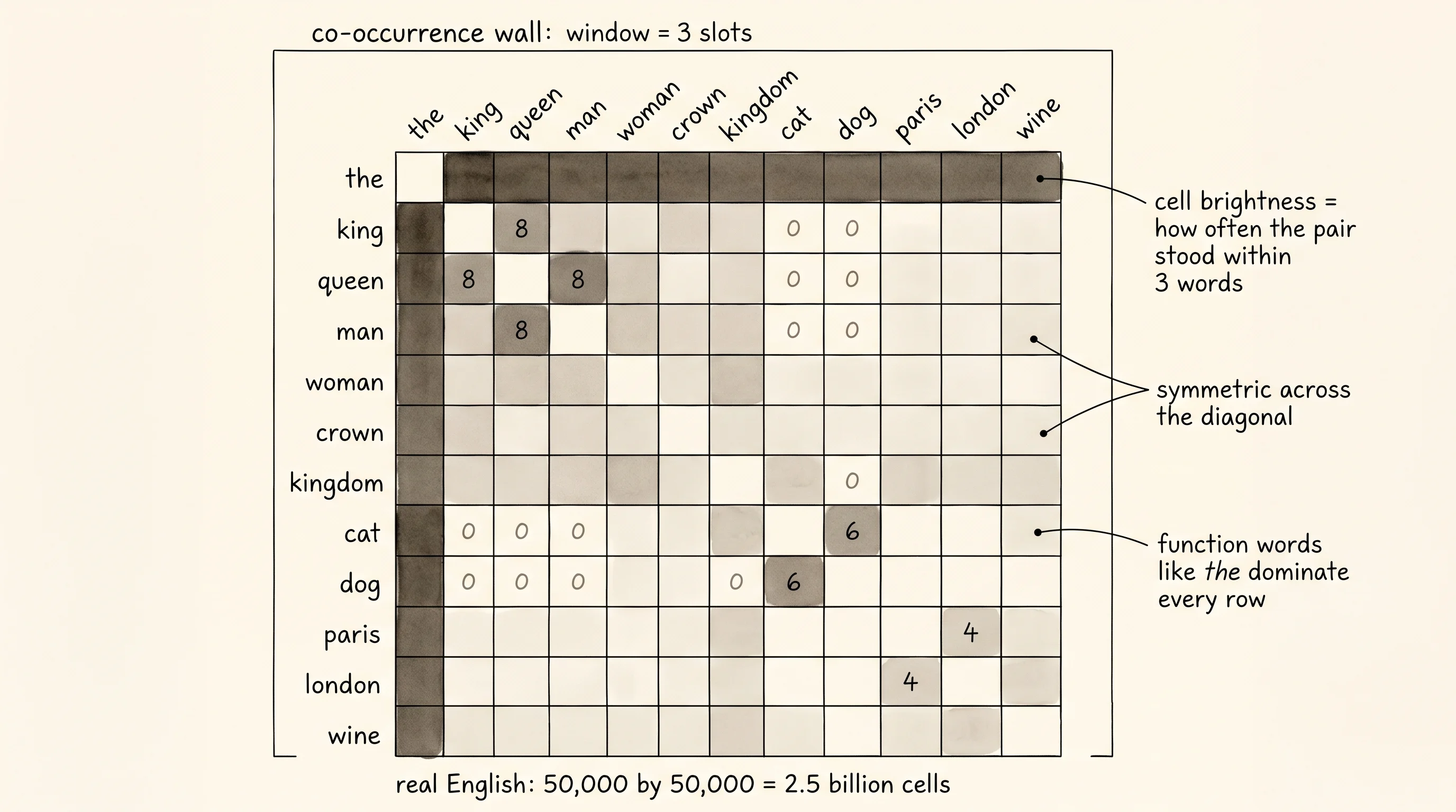
The picture on the wall is a square grid. Words run down the left side and across the top in the same order. Each cell answers one question: how many times did the row word and the column word appear within 3 slots of each other across the whole corpus? "The" and "king" share lots of cells lit up because every sentence about the king starts with "the king." "King" and "queen" share a bright cell because the corpus mentions them in the same sentence over and over. "King" and "rabbit" share a dim cell, maybe zero, because nobody in the corpus put them together. The wall has a row for every word and a column for every word. With a vocabulary of 111 words the wall has 12,321 cells. With a vocabulary of 50,000 words — the size of normal English — the wall has 2.5 billion cells. You cannot stare at 2.5 billion cells. You cannot fit them in a brain. The trick is to find a much smaller pile of numbers that, multiplied back together, recovers the wall. Two thin matrices of 16 numbers per word will do it. Each row of the first matrix is the embedding for one word — its spinal column of meaning, distilled out of every neighbor it ever had.

Make a folder called projects/32-word-relationship-discoverer and open main.py. The corpus is 60 short hand-written sentences glued into a list at the top of the file. Sentences about kings and queens, men and women, cats and dogs, and the capitals of a few countries. Tiny on purpose. Real GloVe trained on 6 billion words from Wikipedia and the Common Crawl. This trains on about 600. The relationships have to be obvious enough at this scale to land.

CORPUS = [
    "the king rules the kingdom with a heavy crown",
    "the queen rules the kingdom beside the king",
    "the king is a man who wears a crown",
    "the queen is a woman who wears a crown",
    # ... 56 more sentences in the same shape ...
]

Tokenize by lowercasing and splitting on whitespace. Build the vocabulary by collecting every unique word. Sort it so the row order is stable across runs. Now walk every sentence and count.

def build_cooccurrence(tokenized, window_size):
    counts = Counter()
    for sentence in tokenized:
        for center_position, center_word in enumerate(sentence):
            window_start = max(0, center_position - window_size)
            window_end = min(len(sentence), center_position + window_size + 1)
            for neighbor_position in range(window_start, window_end):
                if neighbor_position == center_position:
                    continue
                neighbor_word = sentence[neighbor_position]
                counts[(center_word, neighbor_word)] += 1
    return dict(counts)

The window is 3 slots on each side. "King" inside "the king rules the kingdom" sees "the," "rules," "the," "kingdom." Every one of those neighbors gets a tally. Loop over every sentence and every center word and the wall fills itself in. Print the 10 brightest pairs and the wall starts to talk back.

(       the, the       ) appears 62 times
(       the, of        ) appears 28 times
(        of, the       ) appears 28 times
(       the, and       ) appears 20 times
(       and, the       ) appears 20 times
(       the, a         ) appears 19 times
(         a, the       ) appears 19 times
(       the, is        ) appears 18 times
(        is, the       ) appears 18 times
(       the, king      ) appears 16 times

The function words dominate the top. "The" sits next to "the" 62 times because the corpus is full of phrases like "the king and the queen." That is fine. The interesting structure is buried in the middle of the wall, where "king" and "queen" pop up next to each other 8 times and "cat" and "dog" pop up next to each other 6 times.

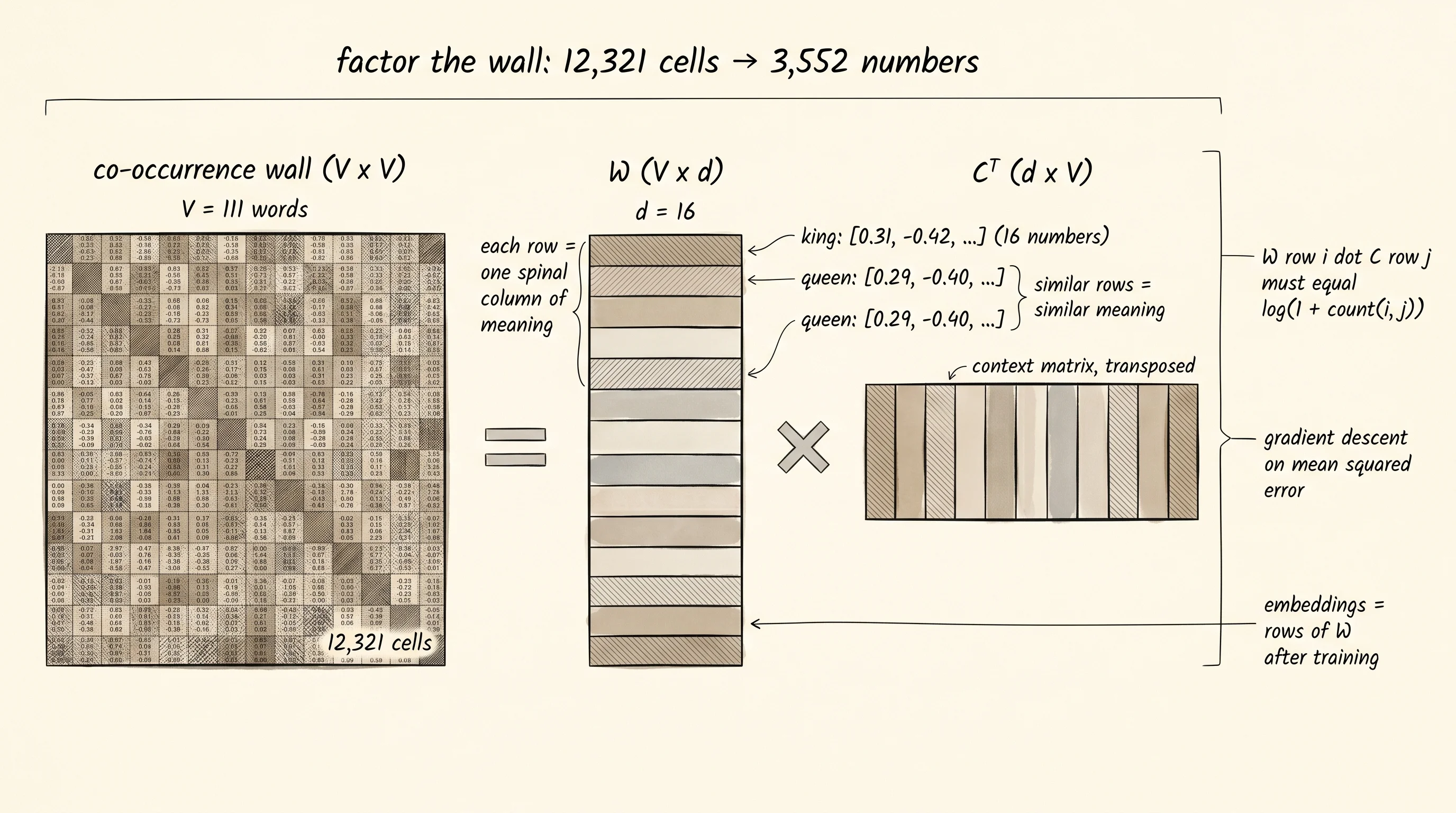
Now the factorization. Pick an embedding dimension — 16 numbers per word. Make two matrices. The first matrix W has one row per word, 16 columns per row. The second matrix C has the same shape. The factorizer's promise is that the dot product of row i of W and row j of C will reconstruct the wall's cell at row i, column j. The wall has 12,321 cells. The two matrices together hold 111 times 16 times 2, or 3,552 numbers. The wall is being squeezed into a quarter of its size. That squeeze is the whole point. The 16 numbers in row i of W are forced to summarize every neighbor word i ever had, because the same row has to participate in the dot products that reconstruct every column of the wall at once. There is nowhere else for the meaning to live.

class MatrixFactorizer:
    def __init__(self, vocab_size, embedding_dim, rng):
        scale = 0.5 / math.sqrt(embedding_dim)
        self.W = [
            [rng.gauss(0.0, scale) for _ in range(embedding_dim)]
            for _ in range(vocab_size)
        ]
        self.C = [
            [rng.gauss(0.0, scale) for _ in range(embedding_dim)]
            for _ in range(vocab_size)
        ]

The target you fit is not the raw count. It is the log of 1 plus the count. The log keeps the function words from drowning out the signal — without it, "the" next to "the" with a count of 62 contributes more loss than the next 100 pairs combined. The plus 1 keeps the log of zero from blowing up when a pair never co-occurred. This is the same trick GloVe uses, with a slightly fancier weighting curve. For 600 tokens, log of 1 plus count is enough.

The loss is mean squared error on the log counts. For one pair (i, j) with target t, the prediction is the dot product of W row i and C row j, and the loss is half the squared error. Because the only operation is a dot product, the gradients are short. The gradient on W row i is the error times C row j, and the gradient on C row j is the error times W row i. Plain SGD: subtract the learning rate times the gradient.

def train(factorizer, training_pairs, learning_rate, epochs, print_every, rng):
    loss_curve = []
    pairs = list(training_pairs)
    for epoch in range(1, epochs + 1):
        rng.shuffle(pairs)
        epoch_loss = 0.0
        for center_index, context_index, target in pairs:
            center_vector = factorizer.W[center_index]
            context_vector = factorizer.C[context_index]
            prediction = dot_product(center_vector, context_vector)
            error = prediction - target
            epoch_loss += 0.5 * error * error
            for k in range(factorizer.embedding_dim):
                gradient_w = error * context_vector[k]
                gradient_c = error * center_vector[k]
                center_vector[k] -= learning_rate * gradient_w
                context_vector[k] -= learning_rate * gradient_c
        average_loss = epoch_loss / len(pairs)
        loss_curve.append(average_loss)
        if epoch == 1 or epoch % print_every == 0:
            print(f"epoch {epoch:4d} | loss {average_loss:.5f}")
    return loss_curve

Run 300 epochs at a learning rate of 0.05. Watch the loss collapse.

epoch    1 | loss 0.61098
epoch   50 | loss 0.00083
epoch  100 | loss 0.00009
epoch  150 | loss 0.00002
epoch  200 | loss 0.00001
epoch  250 | loss 0.00001
epoch  300 | loss 0.00000

The loss going to zero means W times C transposed has reproduced the wall to nearly full precision. The 3,552 numbers really do encode the 12,321 cells. The squeeze worked. Now the rows of W are the embeddings — the spinal columns of meaning the lesson promised. A word's embedding is a list of 16 numbers, and the only thing you can do with a list of 16 numbers is compare it to another list of 16 numbers.

The standard comparison is cosine similarity. Take the dot product of the two vectors and divide by the product of their lengths. The result is between negative 1 and positive 1. A score near 1 means the two words point the same direction in embedding space. A score near 0 means they are unrelated. A score near negative 1 means they are opposites.

def cosine_similarity(a, b):
    norm_a = vector_norm(a)
    norm_b = vector_norm(b)
    if norm_a == 0.0 or norm_b == 0.0:
        return 0.0
    return dot_product(a, b) / (norm_a * norm_b)

Print the top 3 nearest neighbors for a few hand-picked words. The whole point of the exercise is that the neighbors should match human intuition about meaning, not about spelling.

      king -> queen (+0.932), full (+0.787), boy (+0.768)
     queen -> king (+0.932), runs (+0.806), dragon (+0.788)
       cat -> dog (+0.871), girl (+0.729), beside (+0.718)
       dog -> cat (+0.871), is (+0.753), beside (+0.684)
     paris -> walks (+0.816), london (+0.784), by (+0.730)

Read the table. The closest word to "king" is "queen" at 0.932. The closest word to "queen" is "king" at the same score. Cat and dog are each other's closest neighbor at 0.871. Paris and London land near each other. The corpus never said "king is similar to queen" anywhere. The model figured it out because in 60 sentences "king" and "queen" stood next to almost the same set of neighbor words — the same kingdoms, the same crowns, the same feasts. Same neighbors, same column of W. Distributional semantics in 300 epochs.

The famous test is the analogy. Take "king" minus "man" plus "woman" and find the nearest word in the embedding space. If the embeddings encoded the gender direction, the answer should be "queen." Build the target vector with vector arithmetic and search.

def analogy(word_a, word_b, word_c, vocab, index_of, embeddings):
    excluded = {word_a, word_b, word_c}
    target_vector = vector_add(
        vector_subtract(embeddings[index_of[word_b]], embeddings[index_of[word_a]]),
        embeddings[index_of[word_c]],
    )
    best_word = ""
    best_score = -2.0
    for candidate_index, candidate_word in enumerate(vocab):
        if candidate_word in excluded:
            continue
        score = cosine_similarity(target_vector, embeddings[candidate_index])
        if score > best_score:
            best_score = score
            best_word = candidate_word
    return best_word, best_score

Run a handful of queries.

   man -> king   ::  woman -> queen      (cos +0.926)
  king -> queen  :: prince -> cup        (cos +0.840)
 paris -> france :: london -> cup        (cos +0.732)
   cat -> milk   ::    dog -> given      (cos +0.676)
   man -> boy    ::  woman -> girl       (cos +0.855)

The first query lands. Man is to king as woman is to queen, and the model found it on its own from 60 sentences. The fifth lands too: man is to boy as woman is to girl. The middle three miss — the corpus is too small for the gender-and-royalty axis to also encode the parent-and-child axis or the country-and-capital axis. Real GloVe gets all of them right because real GloVe trained on 6 billion tokens. The lesson is that the recipe is correct at any scale. More data and the same gradient-descent loop turns into the embedding tables that GPT and Claude read on every single token they ever process.

A small question to answer from the run. The corpus never contains the sentence "the king is similar to the queen." It never says "kings and queens are related." How did the model decide they belong next to each other? Because every neighbor word "king" appeared next to — kingdom, crown, rules, feast, wine — appeared next to "queen" at almost the same rate. The two words share a column of company. The 16-number embedding of "king" had to land near the 16-number embedding of "queen" for the dot products with "kingdom" and "crown" to come out the same. The structure of the wall forced the structure of the columns.

Embeddings are the input to the brain. The brain still needs a way to decide which embeddings to focus on at any moment.