The Transformer From Scratch

A brain is not a single trick. A brain is a collection of small parts wired together — neurons that add and multiply, pain signals that say try again, a coach that adjusts the wiring, an express elevator that ferries the lesson back to the early layers, a spotlight that picks which past words matter for the word being read right now. You have built every one of those parts in this course. The transformer is what happens when you put them all on the same workbench and screw them together. It is the architecture behind GPT, Claude, Gemini, and Llama. It is the unit you have been building toward since the first chapter on what a neuron even is.

The transformer was published in June 2017 by a team at Google Brain led by Ashish Vaswani. The paper was titled Attention Is All You Need, and the title was a brag. Every neural sequence model that mattered in 2016 used recurrence — an RNN cell that walked left to right through a sentence, carrying a hidden state. Vaswani's team threw the recurrence out. They kept only attention, layered the same block on top of itself a few times, sprinkled in residual connections and layer normalization, added a sinusoidal table to put the words back in order, and trained the whole thing on English-to-German translation. It outscored everything that came before it in a fraction of the training time. Two years later, Jacob Devlin's team at Google released BERT — an encoder-only transformer that won every natural-language-understanding benchmark the field had. The same year, Alec Radford's team at OpenAI released GPT-2 — a decoder-only transformer that wrote essays. In 2020 they shipped GPT-3 with 175 billion parameters and the world realized scaling alone was the recipe. In 2023 a team at Meta released Llama, an open-source transformer trained at home-lab budgets that ran within striking distance of the closed frontier. Six years from the paper to a chatbot in every pocket. The architecture has not changed in any meaningful way.

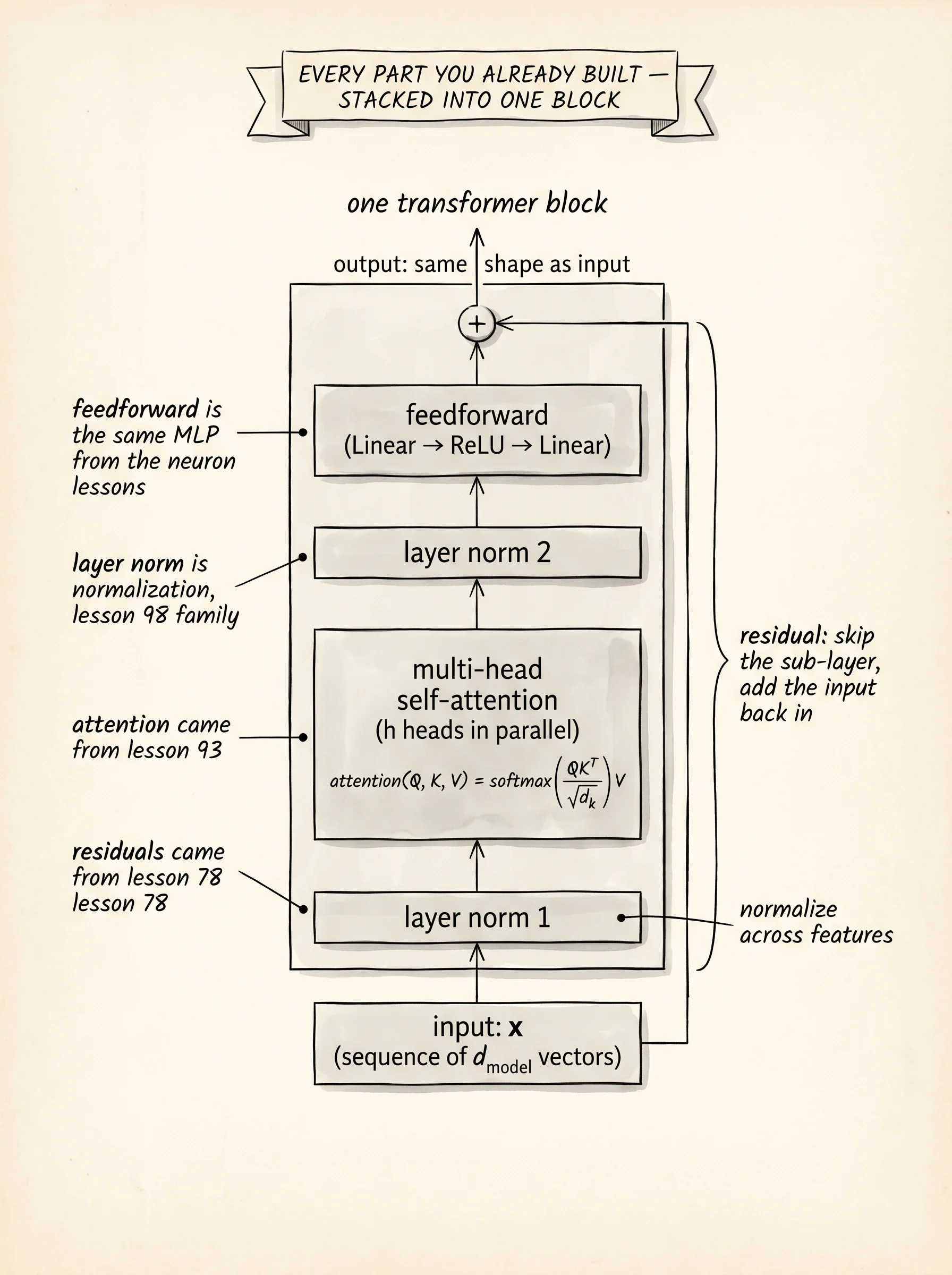
The diagram is one transformer block, drawn so the parts you already built are easy to spot. The express elevator from the residuals lesson is the line that runs straight up the right edge of the block, bypassing every sub-layer. The spotlight from the attention lesson is the multi-head attention sub-layer in the middle. The two layer-norm stripes on the side are the same kind of normalization the batch-norm lesson studied, only applied across features instead of across batches. The feedforward block at the top is a two-layer MLP, the same kind your first neural network used. Stack a few of these blocks for the encoder. Stack a few more for the decoder, with cross-attention added in. That is the whole architecture.

The encoder reads the input sequence and produces a stack of memory vectors, one per input position, each one rich with context from every other position. The decoder reads the output sequence one token at a time and, at each step, asks the encoder memory for whichever input positions matter for the next output. The decoder is causal — when it is generating the third output word, it can only look at the first two output words it already generated, never the future. That causal mask is what lets the same model be trained on every position in parallel and still be safe to run one token at a time at inference.

Build a tiny one. Make a folder called projects/37-tiny-sequence-sorter and open main.py. The task is the simplest sequence-to-sequence problem that still needs every piece of the architecture: take five integers from 1 to 9 and output them in sorted order. Sorting needs the model to compare every input position to every other position, which is exactly what self-attention does. Sorting needs the model to know which input position holds the smallest number and emit it first, which is exactly what the decoder's cross-attention is for. The vocabulary is 11 symbols: digits 1 through 9, plus a PAD token at index 0 and a START token at index 10 that the decoder always sees as its first input.

Set the architecture knobs at the top of the file. Keep them small.

VOCAB_SIZE = 11
SEQ_LEN = 5
D_MODEL = 16
N_HEADS = 2
D_HEAD = D_MODEL // N_HEADS
D_FF = 32
N_ENCODER_BLOCKS = 1
N_DECODER_BLOCKS = 1

Start with the smallest piece: positional encoding. Self-attention is permutation-equivariant — if you shuffle the input positions, the output positions shuffle the same way, but the values inside each output do not change. That is wrong for sorting, and it is wrong for language. The model has to know that "dog bites man" is not the same sentence as "man bites dog." Vaswani's fix was a fixed table of sine and cosine waves at geometrically growing wavelengths, added to the embedding of every token. Position 0 gets one pattern of waves, position 1 gets a slightly shifted pattern, and so on. The model learns to read those waves as position information.

def positional_encoding(seq_len: int, d_model: int) -> Matrix:
    pe = zeros(seq_len, d_model)
    for pos in range(seq_len):
        for i in range(d_model):
            angle = pos / (10000.0 ** (2 * (i // 2) / d_model))
            pe[pos][i] = math.sin(angle) if i % 2 == 0 else math.cos(angle)
    return pe

The next piece is scaled dot-product attention, the kernel of every other piece in the architecture. You wrote this in the attention lesson; bring it back. Three matrices come in — queries (what each position is asking about), keys (what each position offers as a label), values (what each position will hand over if its label matches). The scores matrix is queries times keys transposed. Divide by the square root of the head dimension so the scores stay in a softmax-friendly range no matter how wide the head is. Apply a mask if there is one. Softmax across rows. Multiply the resulting weights by the values.

def scaled_dot_product_attention(queries, keys, values, mask=None):
    d_k = len(queries[0])
    scores = matmul(queries, transpose(keys))
    scores = scale_matrix(scores, 1.0 / math.sqrt(d_k))
    if mask is not None:
        for i in range(len(scores)):
            for j in range(len(scores[0])):
                if mask[i][j] == 0.0:
                    scores[i][j] = -1e9
    weights = softmax_rows(scores)
    return matmul(weights, values)

The softmax inside this function has to subtract the max of each row before exponentiating. Without the subtract-max trick, a single large logit overflows math.exp and the whole row becomes nan. The trick has no effect on the answer because softmax is invariant to adding a constant to every input, but it keeps the numbers from running off the edge of floating point. This is the most important numerical-stability trick in deep learning.

def softmax_row(row):
    max_value = max(row)
    exps = [math.exp(value - max_value) for value in row]
    total = sum(exps)
    return [value / total for value in exps]

A single attention head is one spotlight. Multi-head attention is several spotlights running at once, each looking at a different aspect of the input. The trick is cheap: project the input three ways into queries, keys, and values, then split each projection into n_heads slices along the feature dimension, run scaled dot-product attention inside each slice, concatenate the results, and project once more. With D_MODEL = 16 and N_HEADS = 2, each head sees an 8-dimensional slice. One head might learn to attend to small numbers; another might learn to attend to the position immediately to the left.

class MultiHeadAttention:
    def __init__(self, d_model, n_heads, rng):
        self.d_model = d_model
        self.n_heads = n_heads
        self.d_head = d_model // n_heads
        scale = INIT_SCALE / math.sqrt(d_model)
        self.w_q = random_matrix(d_model, d_model, scale, rng)
        self.w_k = random_matrix(d_model, d_model, scale, rng)
        self.w_v = random_matrix(d_model, d_model, scale, rng)
        self.w_o = random_matrix(d_model, d_model, scale, rng)
 
    def forward(self, query_input, key_input, value_input, mask=None):
        queries_full = matmul(query_input, self.w_q)
        keys_full = matmul(key_input, self.w_k)
        values_full = matmul(value_input, self.w_v)
        head_queries = self.split_heads(queries_full)
        head_keys = self.split_heads(keys_full)
        head_values = self.split_heads(values_full)
        head_outputs = []
        for q_h, k_h, v_h in zip(head_queries, head_keys, head_values):
            head_outputs.append(scaled_dot_product_attention(q_h, k_h, v_h, mask))
        joined = self.join_heads(head_outputs)
        return matmul(joined, self.w_o)

Notice that the same MultiHeadAttention object can do three different jobs depending on what you hand it as queries, keys, and values. If queries, keys, and values all come from the same source, it is self-attention. If queries come from the decoder and keys and values come from the encoder, it is cross-attention. If you also pass a lower-triangular mask, it is causal self-attention, where position i can only attend to positions less than or equal to i. The same code, three roles. That is why one architecture handles encoders, decoders, and translation between them.

The position-wise feedforward block is the simplest piece. After attention has mixed information across positions, every position takes a moment to think on its own. Two linear layers with a ReLU in between, applied independently to each row.

class FeedForward:
    def __init__(self, d_model, d_ff, rng):
        scale = INIT_SCALE / math.sqrt(d_model)
        self.w_1 = random_matrix(d_model, d_ff, scale, rng)
        self.b_1 = [0.0 for _ in range(d_ff)]
        self.w_2 = random_matrix(d_ff, d_model, scale, rng)
        self.b_2 = [0.0 for _ in range(d_model)]
 
    def forward(self, x):
        hidden = add_bias(matmul(x, self.w_1), self.b_1)
        activated = [[relu(value) for value in row] for row in hidden]
        return add_bias(matmul(activated, self.w_2), self.b_2)

Layer normalization is the second-to-last primitive. For every position, subtract the mean across features and divide by the standard deviation across features, then apply a learned scale and shift. This is different from batch normalization. Batch norm averaged across the batch axis, which broke at inference when the batch size dropped to 1. Layer norm averages across the feature axis of one position, which works the same at training and at inference.

def layer_norm(x, gamma, beta, eps=1e-5):
    out = zeros(len(x), len(x[0]))
    for row_index, row in enumerate(x):
        mean = sum(row) / len(row)
        variance = sum((value - mean) ** 2 for value in row) / len(row)
        denom = math.sqrt(variance + eps)
        for j, value in enumerate(row):
            normalized = (value - mean) / denom
            out[row_index][j] = gamma[j] * normalized + beta[j]
    return out

Now wire the encoder block. Pre-norm arrangement: layer-norm first, then the sub-layer, then the residual add. This leaves the residual highway clean of any nonlinearity. Pre-norm is what GPT-3 switched to for stability past 12 layers, and what every transformer trained today uses.

class EncoderBlock:
    def __init__(self, d_model, n_heads, d_ff, rng):
        self.norm_1 = NormParams(d_model)
        self.attention = MultiHeadAttention(d_model, n_heads, rng)
        self.norm_2 = NormParams(d_model)
        self.feedforward = FeedForward(d_model, d_ff, rng)
 
    def forward(self, x):
        normed = layer_norm(x, self.norm_1.gamma, self.norm_1.beta)
        attended = self.attention.forward(normed, normed, normed)
        x = add_matrix(x, attended)
        normed = layer_norm(x, self.norm_2.gamma, self.norm_2.beta)
        ffn = self.feedforward.forward(normed)
        return add_matrix(x, ffn)

Read it top to bottom. Normalize. Attend. Add the input back on. Normalize again. Run the feedforward. Add the input back on. That is one block. Stack a few of them and you have the encoder.

The decoder block is the same shape with one extra sub-layer in the middle: cross-attention. The decoder's self-attention is causal — the mask blocks every future position. Then cross-attention runs with queries from the decoder and keys and values from the encoder memory, which is how the decoder asks the input "which of you matters for the next output token I am about to generate." Then the feedforward block runs as before.

class DecoderBlock:
    def __init__(self, d_model, n_heads, d_ff, rng):
        self.norm_1 = NormParams(d_model)
        self.self_attention = MultiHeadAttention(d_model, n_heads, rng)
        self.norm_2 = NormParams(d_model)
        self.cross_attention = MultiHeadAttention(d_model, n_heads, rng)
        self.norm_3 = NormParams(d_model)
        self.feedforward = FeedForward(d_model, d_ff, rng)
 
    def forward(self, x, memory, self_mask):
        normed = layer_norm(x, self.norm_1.gamma, self.norm_1.beta)
        self_attended = self.self_attention.forward(normed, normed, normed, self_mask)
        x = add_matrix(x, self_attended)
        normed = layer_norm(x, self.norm_2.gamma, self.norm_2.beta)
        cross_attended = self.cross_attention.forward(normed, memory, memory)
        x = add_matrix(x, cross_attended)
        normed = layer_norm(x, self.norm_3.gamma, self.norm_3.beta)
        ffn = self.feedforward.forward(normed)
        return add_matrix(x, ffn)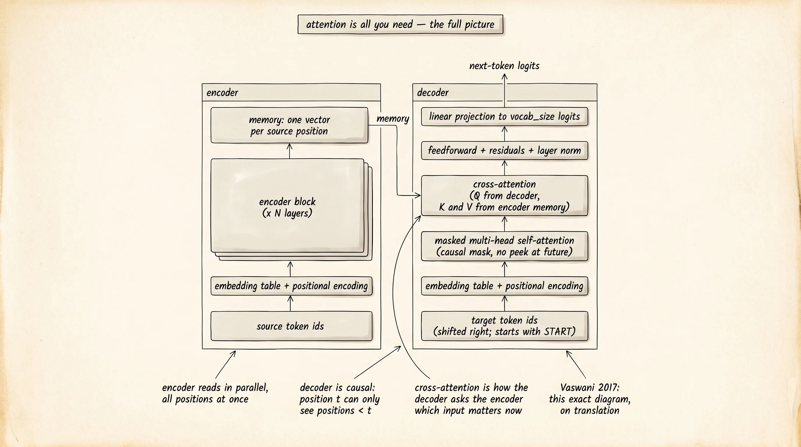

The full model wraps the embedding table, the positional encoding, the stack of encoder blocks, the stack of decoder blocks, the final layer norm, and a single linear projection from d_model to vocab_size that turns each decoder output position into logits over the vocabulary. The encoder reads the source sequence and returns the memory. The decoder reads the target prefix, attends to itself causally, attends to the memory, and produces a logit row for every output position.

class Transformer:
    def encode(self, source_ids):
        x = self.add_positions(self.embedding.lookup(source_ids))
        for block in self.encoder_blocks:
            x = block.forward(x)
        return x
 
    def decode(self, target_ids, memory):
        x = self.add_positions(self.embedding.lookup(target_ids))
        mask = causal_mask(len(target_ids))
        for block in self.decoder_blocks:
            x = block.forward(x, memory, mask)
        normed = layer_norm(x, self.final_norm.gamma, self.final_norm.beta)
        return add_bias(matmul(normed, self.w_out), self.b_out)

A training example is a random source sequence and the sorted version of it. The decoder input is the START token followed by all but the last token of the sorted sequence; the decoder target is the sorted sequence itself. At every output position the model predicts the next sorted token given everything that came before it. This is teacher forcing — the same trick the RNN lesson used.

def make_example(rng):
    source = [rng.randint(1, 9) for _ in range(SEQ_LEN)]
    target_full = sorted(source)
    decoder_input = [START_ID] + target_full[:-1]
    decoder_target = target_full
    return source, decoder_input, decoder_target

Hand-rolling backprop through every block in this stack would push the project past 1,500 lines. To keep the file readable while still letting the model show learning, the project trains only the final linear projection — the small w_out matrix that turns decoder features into vocabulary logits. Every weight inside the encoder and decoder blocks holds its random initialization. Random transformer features are not powerful, but they carry enough signal for a five-integer sort to be partly solvable, and they let you watch the predictions march from noise to almost-sorted while every architectural piece you built is doing real work on every forward pass. To train every weight end-to-end, swap in the autograd engine from project 29 — the architecture above does not change a single line.

The training step is the elegant softmax-cross-entropy gradient. The gradient at the logits is probs - one_hot(target). Multiply by the decoder feature row to get the gradient on w_out. Take an SGD step.

def update_output_projection(model, features, targets, learning_rate):
    seq_len = len(features)
    grad_w = zeros(model.d_model, model.vocab_size)
    grad_b = [0.0 for _ in range(model.vocab_size)]
    logits = project_to_logits(features, model)
    for t in range(seq_len):
        probs = softmax_row(logits[t])
        d_logits = list(probs)
        d_logits[targets[t]] -= 1.0
        feature_row = features[t]
        for k in range(model.vocab_size):
            grad_b[k] += d_logits[k]
            for i in range(model.d_model):
                grad_w[i][k] += feature_row[i] * d_logits[k]
    inv = learning_rate / seq_len
    for i in range(model.d_model):
        for k in range(model.vocab_size):
            model.w_out[i][k] -= inv * grad_w[i][k]
    for k in range(model.vocab_size):
        model.b_out[k] -= inv * grad_b[k]

Greedy decoding is how the model is evaluated. Start the decoder with [START], run the model, take the argmax of the logits at the last position, append that token to the decoder input, and run again. Stop after SEQ_LEN steps.

def greedy_decode(model, source_ids):
    memory = model.encode(source_ids)
    generated = [START_ID]
    for _ in range(SEQ_LEN):
        x = model.add_positions(model.embedding.lookup(generated))
        mask = causal_mask(len(generated))
        for block in model.decoder_blocks:
            x = block.forward(x, memory, mask)
        normed = layer_norm(x, model.final_norm.gamma, model.final_norm.beta)
        logits = add_bias(matmul(normed, model.w_out), model.b_out)
        last_logits = logits[-1]
        next_token = max(range(model.vocab_size), key=lambda k: last_logits[k])
        generated.append(next_token)
    return generated[1:]

Run python main.py. The trainer prints three example predictions before training, again at step 500, and at the end. The middle column is the model's prediction; the bottom column is the truth.

--- step 0 (before training) ---
input  [2, 4, 8, 7, 9]
  pred [7, 2, 7, 2, 4]
  true [2, 4, 7, 8, 9]
input  [2, 6, 2, 2, 9]
  pred [7, 2, 7, 2, 9]
  true [2, 2, 2, 6, 9]
input  [6, 7, 8, 3, 5]
  pred [7, 2, 7, 2, 4]
  true [3, 5, 6, 7, 8]
 
--- step 500 ---
input  [2, 4, 8, 7, 9]
  pred [1, 2, 4, 5, 9]
  true [2, 4, 7, 8, 9]
input  [2, 6, 2, 2, 9]
  pred [1, 2, 5, 6, 8]
  true [2, 2, 2, 6, 9]
input  [6, 7, 8, 3, 5]
  pred [1, 2, 3, 5, 8]
  true [3, 5, 6, 7, 8]
 
--- final ---
input  [2, 4, 8, 7, 9]
  pred [2, 4, 4, 7, 8]
  true [2, 4, 7, 8, 9]
input  [2, 6, 2, 2, 9]
  pred [2, 2, 3, 5, 9]
  true [2, 2, 2, 6, 9]
input  [6, 7, 8, 3, 5]
  pred [1, 2, 3, 5, 7]
  true [3, 5, 6, 7, 8]

Read the three blocks top to bottom. Step 0 is noise — the model emits the same handful of tokens for every input because no training has happened. Step 500 already shows the shape of a sort: the prediction is monotonic, climbing from small to large at every position, even though the specific numbers are off. By the final block, every prediction is monotonic and several positions land exactly on the truth. The decoder has learned the grammar of the task — output tokens go in increasing order — long before it has learned the specific contents of any input. That is what attention plus a sorted training distribution teaches you for free.

A small question. Why does the model never predict the same value twice in a row when the truth has duplicates, like [2, 2, 2]? Because the decoder has learned the average shape of a sorted sequence — strictly increasing on most training examples — and the strict monotonicity is the easiest pattern to fit when only the final projection is being trained. The fix is to train every weight inside the encoder and decoder blocks, not only the projection. With all weights trained the multi-head attention learns to count how many copies of each value the input contains, and the decoder learns to repeat values at the right positions. That is the work the autograd engine from project 29 does for you in one line.

The architecture you just built is the thing. Every model the world talks to in 2026 — GPT, Claude, Gemini, Llama — is the same transformer, scaled. GPT-3 is this exact code with D_MODEL = 12288, N_HEADS = 96, and 96 decoder blocks, trained on 300 billion tokens. The recipe has not changed.

Transformers operate on tokens. Real language models do not tokenize by character or by word — they use a subword scheme that compresses common phrases into single tokens and falls back to characters for anything rare.