Build an ETL Pipeline

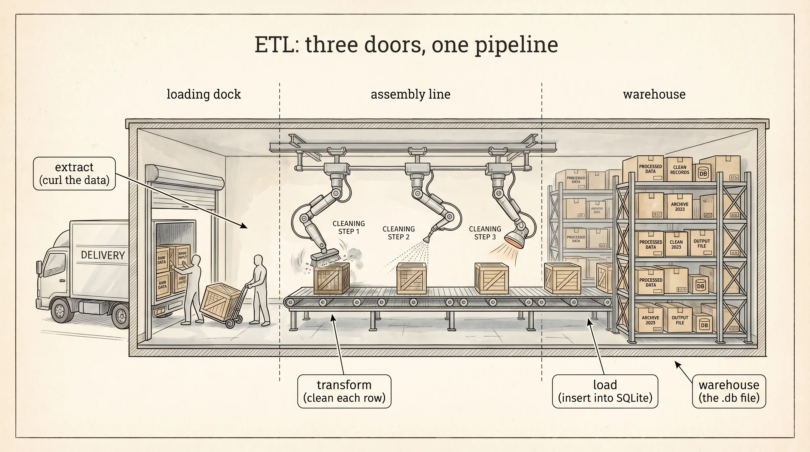
A factory takes raw material in one door and ships finished product out the other. In between sits an assembly line that cuts, cleans, and stamps. ETL is the same three-door shape for data. Extract pulls the raw material from somewhere you do not own. Transform runs the assembly line that cleans the junk. Load puts the finished rows on the warehouse shelf where your own code can find them. Three scripts, one pipeline.

The pattern came out of IBM mainframe shops in the 1970s. Companies had sales data in one system, inventory in another, and payroll in a third, each with its own format. A nightly job copied the data out, reshaped it, and dropped it into a single reporting database — the first data warehouses. In 2006 a Yahoo engineer named Doug Cutting open-sourced Hadoop and the cheap disk era let teams flip the order: load first, transform later (ELT). In 2014 Maxime Beauchemin at Airbnb wrote Airflow to schedule thousands of these pipelines and handed it to the world. Whatever the buzzword, the shape underneath is still three doors.

The raw material for this lesson is a Spotify dataset — about 170,000 tracks with 19 columns each. Song name, artist, release year, tempo, danceability, energy, popularity, whether the lyrics are marked explicit. The file lives on GitHub. Open your venv and make a project folder for the factory.

cd ~/learning-python
mkdir etl-factory
cd etl-factory

cd $HOME\learning-python
mkdir etl-factory
cd etl-factory

The first door is extract. curl is a tool that speaks HTTP from the command line. It was written by a Swedish engineer named Daniel Stenberg in 1997 so his IRC bot could fetch currency exchange rates. It ships on every Mac, every Linux server, and recent versions of Windows. Point it at a URL and it downloads the bytes to disk.

curl -L -o tracks_raw.csv https://raw.githubusercontent.com/gabminamedez/spotify-data/master/data.csv
ls -lh tracks_raw.csv

curl.exe -L -o tracks_raw.csv https://raw.githubusercontent.com/gabminamedez/spotify-data/master/data.csv
Get-ChildItem tracks_raw.csv

The -L flag tells curl to follow redirects. The -o flag names the output file. After the download you should see a file around 20 MB. The raw material is on the loading dock. Nothing has been cleaned yet.

Write an extract script that reads the first few rows so you can see what the factory is about to process. Save this as extract.py.

import csv
from pathlib import Path
 
raw_path = Path("tracks_raw.csv")
row_count = 0
with open(raw_path, newline="", encoding="utf-8") as handle:
    reader = csv.DictReader(handle)
    header = reader.fieldnames
    print("columns:", header)
    for row in reader:
        row_count += 1
        if row_count <= 3:
            print("sample row:", {k: row[k] for k in ["name", "artists", "year", "tempo", "danceability", "explicit"]})
print("total rows:", row_count)

Run it with python extract.py.

columns: ['valence', 'year', 'acousticness', 'artists', 'danceability', 'duration_ms', 'energy', 'explicit', 'id', 'instrumentalness', 'key', 'liveness', 'loudness', 'mode', 'name', 'popularity', 'release_date', 'speechiness', 'tempo', 'valence']
sample row: {'name': 'Singende Bataillone 1. Teil', 'artists': "['Carl Woitschach']", 'year': '1928', 'tempo': '118.469', 'danceability': '0.708', 'explicit': '0'}
sample row: {'name': 'Fantasiestuecke, Op. 111: Piu tosto lento', 'artists': "['Robert Schumann', 'Vladimir Horowitz']", 'year': '1928', 'tempo': '83.972', 'danceability': '0.379', 'explicit': '0'}
sample row: {'name': 'Chapter 1.18 - Zamek kaniowski', 'artists': "['Seweryn Goszczynski']", 'year': '1928', 'tempo': '80.922', 'danceability': '0.749', 'explicit': '0'}
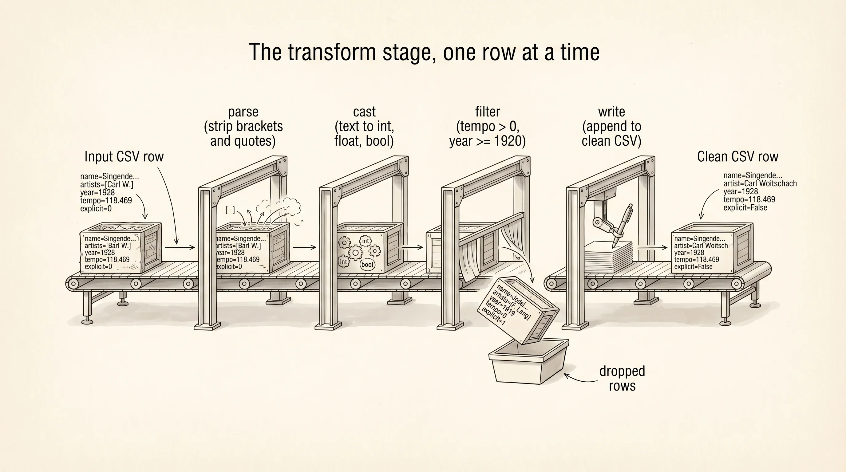
total rows: 169909

The csv.DictReader class ships in Python's standard library. It reads the first line as the column names and hands you every following row as a dictionary keyed by those names. The newline="" keeps Python from double-counting carriage returns on Windows. The sample rows show the mess the assembly line has to deal with. The artists field is a string that looks like a Python list but is actually text — "['Carl Woitschach']" with the brackets and quotes included. The year field is a string. The explicit field is the string "0" or "1", not a boolean. Every number in a CSV is text on disk. The transform stage is where text becomes data.

Write transform.py next to your extract script. The job is to read the raw CSV, clean each row, keep only the columns you care about, and write a smaller CSV that the load stage can trust.

import csv
from pathlib import Path
 
raw_path = Path("tracks_raw.csv")
clean_path = Path("tracks_clean.csv")
 
wanted = ["name", "artist", "year", "tempo", "danceability", "energy", "popularity", "explicit"]
 
def parse_artist(field):
    stripped = field.strip("[]")
    first = stripped.split(",")[0]
    return first.strip().strip("'").strip('"')
 
kept = 0
dropped = 0
with open(raw_path, newline="", encoding="utf-8") as src, \
     open(clean_path, "w", newline="", encoding="utf-8") as dst:
    reader = csv.DictReader(src)
    writer = csv.DictWriter(dst, fieldnames=wanted)
    writer.writeheader()
    for row in reader:
        try:
            clean = {
                "name": row["name"].strip(),
                "artist": parse_artist(row["artists"]),
                "year": int(row["year"]),
                "tempo": float(row["tempo"]),
                "danceability": float(row["danceability"]),
                "energy": float(row["energy"]),
                "popularity": int(row["popularity"]),
                "explicit": row["explicit"] == "1",
            }
        except (ValueError, KeyError):
            dropped += 1
            continue
        if clean["tempo"] <= 0 or clean["year"] < 1920:
            dropped += 1
            continue
        writer.writerow(clean)
        kept += 1
        if kept <= 3:
            print("clean row:", clean)
 
print("kept:", kept, "dropped:", dropped)

clean row: {'name': 'Singende Bataillone 1. Teil', 'artist': 'Carl Woitschach', 'year': 1928, 'tempo': 118.469, 'danceability': 0.708, 'energy': 0.1950, 'popularity': 0, 'explicit': False}
clean row: {'name': 'Fantasiestuecke, Op. 111: Piu tosto lento', 'artist': 'Robert Schumann', 'year': 1928, 'tempo': 83.972, 'danceability': 0.379, 'energy': 0.0135, 'popularity': 0, 'explicit': False}
clean row: {'name': 'Chapter 1.18 - Zamek kaniowski', 'artist': 'Seweryn Goszczynski', 'year': 1928, 'tempo': 80.922, 'danceability': 0.749, 'energy': 0.1300, 'popularity': 0, 'explicit': False}
kept: 169125 dropped: 784

The transform script is the whole assembly line drawn out. Each row goes through a try block because a bad value in one column should not kill the whole factory — a malformed number raises ValueError, the row gets counted as dropped, and the line keeps moving. The parse_artist helper strips the surrounding brackets and quotes the raw file wraps around the artist list and takes the first name. The year < 1920 filter drops rows with garbage dates. By the end 784 rows out of 169,909 were too broken to use. The clean file on disk has 8 columns instead of 20 and every value has a real Python type.

The third door is load. A warehouse for rows is a database. The one you already have on your machine is SQLite — a single file that holds tables and answers SQL queries, written by Richard Hipp in 2000 for a Navy project and now the most-deployed database on earth, sitting inside every iPhone, every Android, and every Chrome browser. Python's standard library ships a module called sqlite3 that lets you open a SQLite file and talk to it. No install needed.

Write load.py.

import csv
import sqlite3
from pathlib import Path
 
clean_path = Path("tracks_clean.csv")
db_path = Path("warehouse.db")
 
db_path.unlink(missing_ok=True)
connection = sqlite3.connect(db_path)
cursor = connection.cursor()
cursor.execute("""
    CREATE TABLE tracks (
        id INTEGER PRIMARY KEY AUTOINCREMENT,
        name TEXT NOT NULL,
        artist TEXT NOT NULL,
        year INTEGER NOT NULL,
        tempo REAL NOT NULL,
        danceability REAL NOT NULL,
        energy REAL NOT NULL,
        popularity INTEGER NOT NULL,
        explicit INTEGER NOT NULL
    )
""")
 
inserted = 0
with open(clean_path, newline="", encoding="utf-8") as src:
    reader = csv.DictReader(src)
    for row in reader:
        cursor.execute(
            "INSERT INTO tracks (name, artist, year, tempo, danceability, energy, popularity, explicit) VALUES (?, ?, ?, ?, ?, ?, ?, ?)",
            (row["name"], row["artist"], int(row["year"]), float(row["tempo"]),
             float(row["danceability"]), float(row["energy"]),
             int(row["popularity"]), 1 if row["explicit"] == "True" else 0),
        )
        inserted += 1
 
connection.commit()
 
cursor.execute("SELECT name, artist, year, tempo FROM tracks LIMIT 3")
for row in cursor.fetchall():
    print("loaded row:", row)
 
cursor.execute("SELECT COUNT(*) FROM tracks")
print("rows in warehouse:", cursor.fetchone()[0])
connection.close()

loaded row: ('Singende Bataillone 1. Teil', 'Carl Woitschach', 1928, 118.469)
loaded row: ('Fantasiestuecke, Op. 111: Piu tosto lento', 'Robert Schumann', 1928, 83.972)
loaded row: ('Chapter 1.18 - Zamek kaniowski', 'Seweryn Goszczynski', 1928, 80.922)
rows in warehouse: 169125

The CREATE TABLE statement is the shelf blueprint. Every column has a type and a NOT NULL constraint, so a bad row cannot sneak in after transform missed it. The ? marks in the INSERT statement are parameter placeholders — you pass the values as a tuple and sqlite3 escapes them for you, which is the one and only defense against a kind of attack called SQL injection. connection.commit() writes everything to disk. Without the commit the file stays empty. Every stage printed a head sample and a row count so you can see what shipped through each door: 169,909 raw, 169,125 clean, 169,125 loaded. The factory works.

A warehouse full of shelves is only useful if you can ask it questions. Write analyze.py. The first question is a real correlation: does a track's popularity rise with its energy? The second is a fake one: does the average popularity of tracks released in even-numbered years match the average for odd-numbered years?

import sqlite3
import math
from pathlib import Path
 
connection = sqlite3.connect(Path("warehouse.db"))
cursor = connection.cursor()
 
def correlation(xs, ys):
    n = len(xs)
    mean_x = sum(xs) / n
    mean_y = sum(ys) / n
    num = sum((x - mean_x) * (y - mean_y) for x, y in zip(xs, ys))
    den_x = math.sqrt(sum((x - mean_x) ** 2 for x in xs))
    den_y = math.sqrt(sum((y - mean_y) ** 2 for y in ys))
    return num / (den_x * den_y)
 
cursor.execute("SELECT energy, popularity FROM tracks WHERE year >= 2000")
rows = cursor.fetchall()
energies = [r[0] for r in rows]
populars = [r[1] for r in rows]
print("energy vs popularity (2000+):", round(correlation(energies, populars), 3))
 
cursor.execute("SELECT AVG(popularity) FROM tracks WHERE year % 2 = 0")
even_avg = cursor.fetchone()[0]
cursor.execute("SELECT AVG(popularity) FROM tracks WHERE year % 2 = 1")
odd_avg = cursor.fetchone()[0]
print("even-year avg popularity:", round(even_avg, 3))
print("odd-year avg popularity:", round(odd_avg, 3))
print("difference:", round(even_avg - odd_avg, 3))
 
connection.close()

energy vs popularity (2000+): 0.214
even-year avg popularity: 29.874
odd-year avg popularity: 29.691
difference: 0.183

A correlation of 0.214 is real but weak — higher-energy songs released since 2000 do tend to be more popular, and the reason has a mechanism you can explain. Radio stations pick high-energy tracks for daytime play, streaming playlists like "Workout" and "Party" lean energetic, and listeners skip low-energy songs faster on Spotify, which tanks their popularity score. The number has causation behind it.

The second finding has a difference of 0.183 popularity points between tracks released in even years and odd years. The number is not zero. A careless analyst could write a paragraph about it. There is no mechanism. The calendar does not know your song exists. Whether 2019 or 2020 is on the release date has no physical path to whether people press play. The correlation is spurious — a coincidence in a dataset big enough that almost any random split shows a tiny gap. This is the trap every data team falls into at some point and why the next lesson exists.

A question to answer from the output: how would you tell the difference between the two findings without the story I just told? The honest answer is you cannot, from the numbers alone. You need a way to ask: if I ran this same test on 10,000 shuffled versions of the data where I know there is no real effect, how often would I see a difference as big as 0.183? That question is what a p-value answers, and it is what keeps the real pattern and the spurious one from looking the same on the page.

You found a pattern. You do not know if it is random.