PyTorch
A lifter at the gym starts the bar light and adds a plate every set. He is not strong on rep one. He is stronger on rep fifty because his body measured the gap between what he tried and what the bar wanted, and adjusted. A neural network learns the same way. The network starts with random weights, you hand it an input, it produces a guess, you measure the gap between the guess and the truth, and the library walks every weight in the network a tiny step toward the answer. A thousand reps later, the network's guesses are sharp. PyTorch is the library that does the measuring and the stepping for you, so you can spend your time describing the shape of the lifter instead of calculating the math behind every rep.
The lineage runs through a few labs. In 2002 a research group at the Idiap lab in Switzerland led by Ronan Collobert released Torch, a machine-learning library written in C with a Lua scripting layer. Facebook picked it up in 2014 for internal research and hired Soumith Chintala, one of its maintainers. In 2015 a small Japanese startup called Preferred Networks released Chainer, the first major library built around a design called define-by-run: instead of compiling the network graph up front and running data through it, you write ordinary Python code and the library records what you did on the fly. That idea was the breakthrough, because it let a researcher debug a network with print statements and a Python debugger, the way you debug anything else. In 2016 Chintala and his team at Facebook AI Research ported Torch to Python with Chainer's execution model baked in, and they called it PyTorch. Version 1.0 shipped in late 2018. Every major academic lab had switched to it within two years, and in 2022 the Linux Foundation took it over from Meta to keep it vendor-neutral.
Install PyTorch. The CPU-only wheel is fine for everything in this lesson; you only need a GPU when you are training on images or audio. The full install for mac and windows is identical if you stay on CPU.
cd ~/learning-python
source .venv/bin/activate
pip install torch
mkdir torch-intro
cd torch-intro
touch tensors.py
touch mlp.py
cd $HOME\learning-python
.venv\Scripts\Activate.ps1
pip install torch
mkdir torch-intro
cd torch-intro
ni tensors.py
ni mlp.pyA tensor is PyTorch's name for an array. It is the same shape as a NumPy array — a contiguous block of memory with a shape, a dtype, and stride metadata — with two extra pieces: every tensor knows which device it lives on (CPU or GPU), and every tensor can be asked to track the gradient of every operation performed on it. Those two features are what turn an array library into a learning library.
Open tensors.py and type:
import torch

x = torch.tensor([1.0, 2.0, 3.0])
print("x:      ", x)
print("shape:  ", x.shape)
print("dtype:  ", x.dtype)
print("device: ", x.device)

y = x * 2 + 1
print("y:      ", y)

a = torch.tensor(3.0, requires_grad=True)
b = a ** 2 + 2 * a + 1
b.backward()
print("a.grad: ", a.grad)
x: tensor([1., 2., 3.])
shape: torch.Size([3])
dtype: torch.float32
device: cpu
y: tensor([3., 5., 7.])
a.grad: tensor(8.)The first 6 lines mirror NumPy. torch.tensor builds an array. Operations broadcast and vectorize the same way. The interesting lines are the last 4. requires_grad=True tells PyTorch to record every operation that touches a into a graph. b.backward() walks the graph backward from b and computes the derivative of b with respect to every leaf tensor that had requires_grad=True. For b = a² + 2a + 1, the derivative with respect to a is 2a + 2, which at a = 3 is 8. PyTorch computed that derivative without you writing any calculus. That is autograd. Every neural network is a chain of those computations, and backward() is the library's name for the chain rule run from the loss back to every weight.
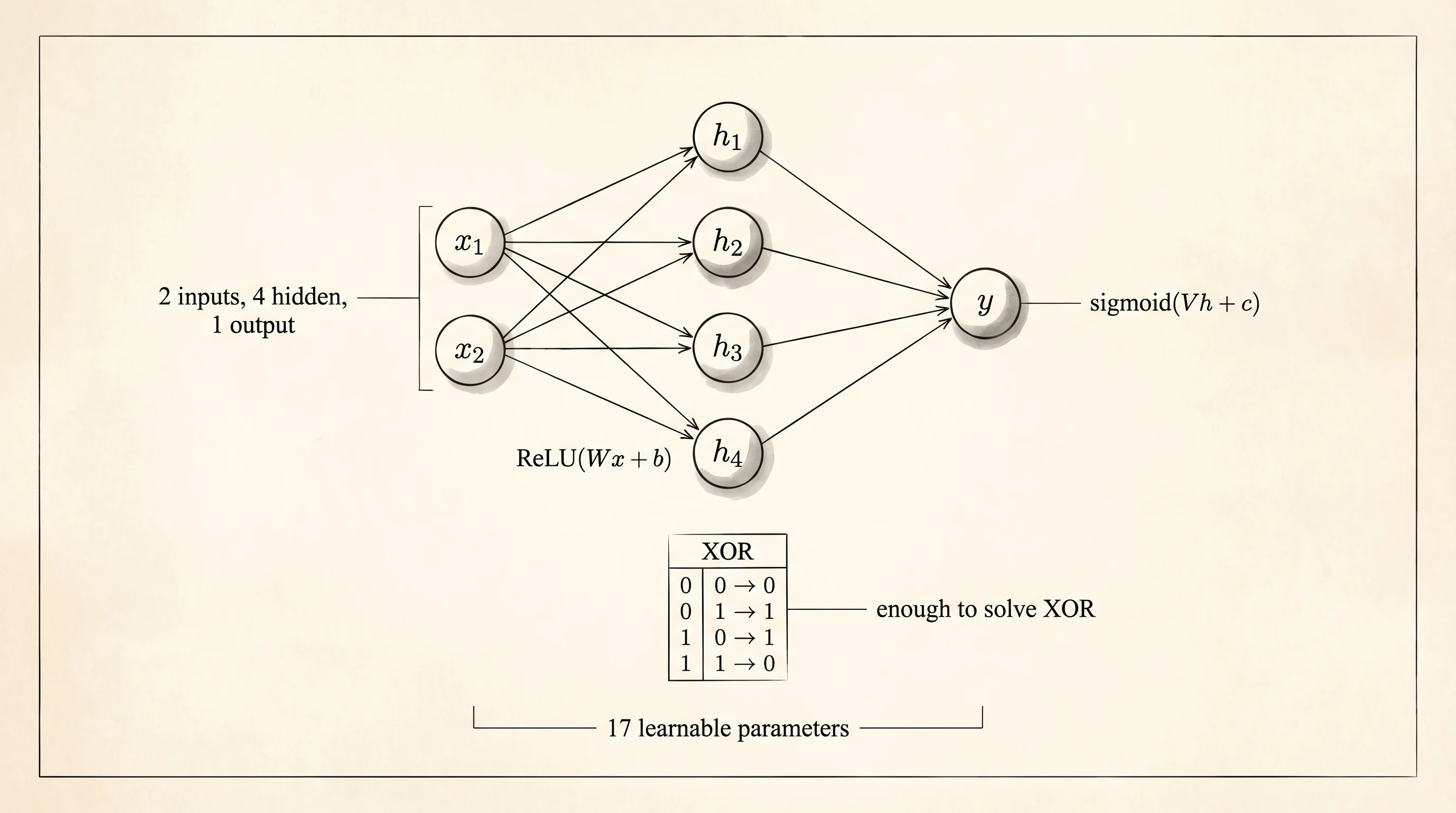
The curriculum asked for a tiny 2-layer MLP trained on a small dataset. MLP means multi-layer perceptron — a network where every layer is a matrix multiply followed by a simple nonlinear function like ReLU. Two layers means two of those stacked. The smallest toy problem that a 2-layer MLP can learn is the XOR function: input is two bits, output is 1 when the bits differ, 0 when they match. XOR is famous in neural network history because a single-layer perceptron cannot solve it, which Marvin Minsky and Seymour Papert proved in their 1969 book and which killed neural network research for a decade. A 2-layer network can.
Open mlp.py and write the whole thing. It is 40 lines, every line does one job.
import torch
import torch.nn as nn
import torch.optim as optim


torch.manual_seed(42)

X = torch.tensor([[0.0, 0.0], [0.0, 1.0], [1.0, 0.0], [1.0, 1.0]])
Y = torch.tensor([[0.0], [1.0], [1.0], [0.0]])


class XorMLP(nn.Module):
    def __init__(self) -> None:
        super().__init__()
        self.layer1 = nn.Linear(2, 4)
        self.layer2 = nn.Linear(4, 1)

    def forward(self, x: torch.Tensor) -> torch.Tensor:
        hidden = torch.relu(self.layer1(x))
        return torch.sigmoid(self.layer2(hidden))


model = XorMLP()
loss_fn = nn.BCELoss()
optimizer = optim.SGD(model.parameters(), lr=0.5)

for epoch in range(1, 2001):
    preds = model(X)
    loss = loss_fn(preds, Y)
    optimizer.zero_grad()
    loss.backward()
    optimizer.step()

    if epoch == 1 or epoch % 250 == 0:
        with torch.no_grad():
            hard = (preds > 0.5).float()
        print(f"epoch {epoch:>4}  loss={loss.item():.4f}  preds={hard.flatten().tolist()}")

with torch.no_grad():
    final = model(X)
print("\nfinal raw outputs:")
for (x, p, y) in zip(X.tolist(), final.flatten().tolist(), Y.flatten().tolist()):
    print(f"  input={x}  pred={p:.3f}  truth={y}")
Run it:
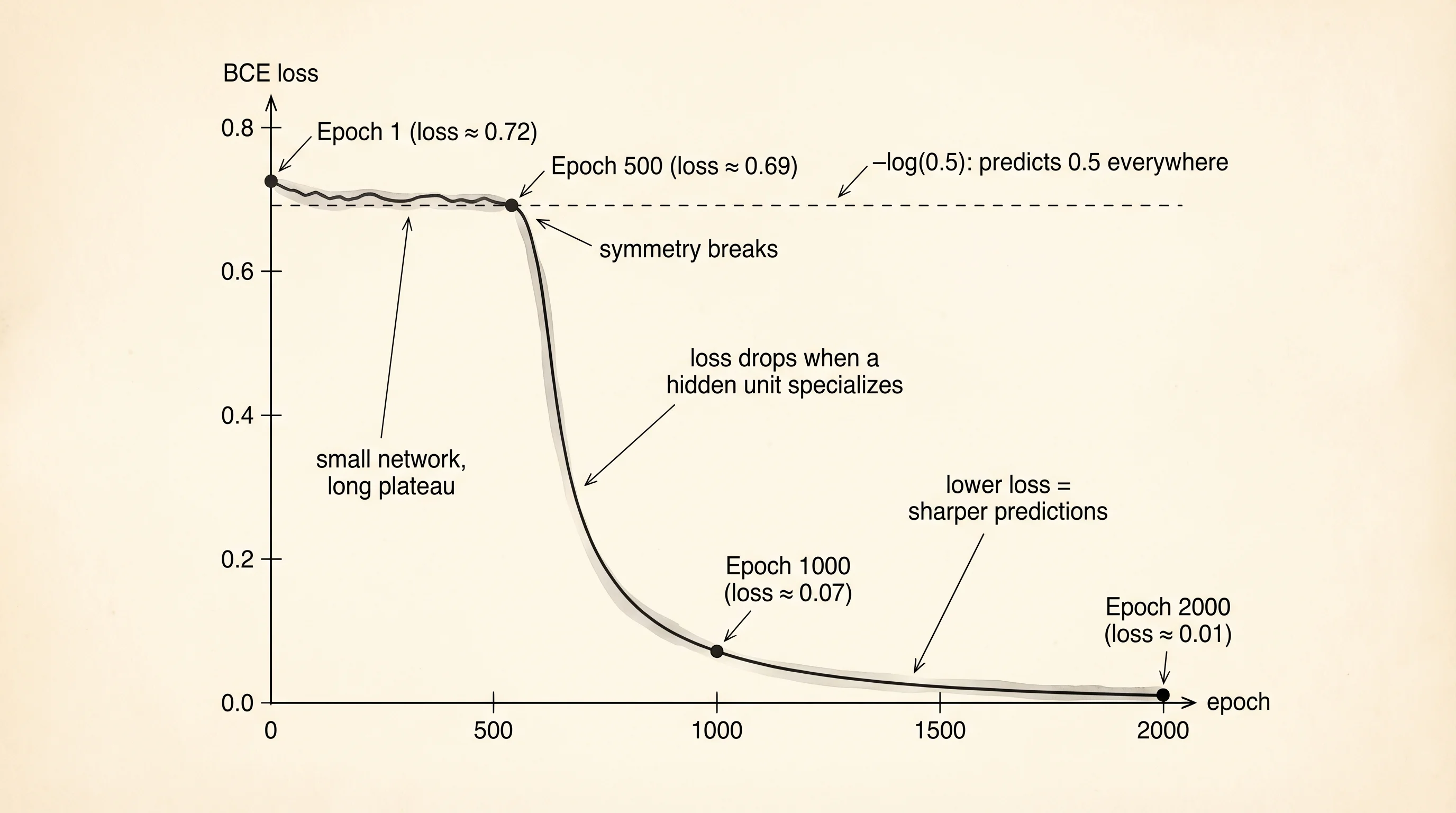
python mlp.pyepoch 1 loss=0.7156 preds=[1.0, 1.0, 1.0, 1.0]
epoch 250 loss=0.6931 preds=[0.0, 0.0, 0.0, 0.0]
epoch 500 loss=0.6819 preds=[0.0, 1.0, 1.0, 0.0]
epoch 750 loss=0.3242 preds=[0.0, 1.0, 1.0, 0.0]
epoch 1000 loss=0.0731 preds=[0.0, 1.0, 1.0, 0.0]
epoch 1250 loss=0.0345 preds=[0.0, 1.0, 1.0, 0.0]
epoch 1500 loss=0.0221 preds=[0.0, 1.0, 1.0, 0.0]
epoch 1750 loss=0.0162 preds=[0.0, 1.0, 1.0, 0.0]
epoch 2000 loss=0.0127 preds=[0.0, 1.0, 1.0, 0.0]
final raw outputs:
input=[0.0, 0.0] pred=0.010 truth=0.0
input=[0.0, 1.0] pred=0.989 truth=1.0
input=[1.0, 0.0] pred=0.988 truth=1.0
input=[1.0, 1.0] pred=0.012 truth=0.0The network learned XOR. Every predicted probability is within 2 percent of the truth. Walk back through the code and see what each line did.
torch.manual_seed(42) locks the random initialization so the run is reproducible; without it the starting weights are different every time and so is the loss curve. X and Y are the dataset — 4 input rows of 2 bits each and 4 target rows of 1 bit each. Real datasets live in the millions; XOR has 4 cases and you keep them all in memory.
class XorMLP(nn.Module) defines the network. Every PyTorch network inherits from nn.Module, which registers the layers as parameters so the optimizer can find them. nn.Linear(2, 4) is a layer with 2 inputs and 4 outputs — a 2x4 weight matrix plus a 4-element bias vector, 12 learnable numbers total. nn.Linear(4, 1) takes those 4 hidden values down to 1 output, 5 more numbers. Total parameter count: 17. forward(self, x) is the method the library calls when you do model(X). Inside, layer1(x) does the matrix multiply and adds the bias, torch.relu zeros out the negatives, layer2 projects to 1 output, and torch.sigmoid squashes the result into (0, 1) so it reads as a probability. That 3-operation chain is the whole network.
nn.BCELoss is binary cross-entropy — the right loss function when the output is a probability of a yes/no label. optim.SGD is plain stochastic gradient descent with learning rate 0.5. Inside the training loop, 4 steps run every epoch. model(X) computes predictions, storing the operation graph. loss_fn(preds, Y) produces a scalar measuring how wrong the predictions are. optimizer.zero_grad() clears the gradient accumulator; PyTorch adds gradients by default, and you have to reset them or they pile up. loss.backward() walks the graph backward and fills every parameter's .grad slot with its derivative of the loss. optimizer.step() reads those grads and nudges every parameter in the direction that reduces the loss.
A question worth answering from the output: the loss hangs near 0.69 from epoch 1 to roughly epoch 500, then drops hard. What happened?
0.69 is -log(0.5) — the loss a model gets when it predicts 0.5 for every input. For the first 500 epochs the network has not yet broken symmetry: the hidden layer weights are small and similar, and every output rounds to 0.5. Once the weights drift far enough for one hidden unit to start firing on (0, 1) and another on (1, 0), the gradient finally has a direction to push in, and the loss cliffs. This is the famous "XOR plateau." Deeper networks with more hidden units escape it in 50 epochs; a 2-layer network with only 4 hidden units takes 500.
A GPU does the same math, wider. A CPU has 8 to 16 cores; a consumer NVIDIA card has several thousand smaller cores. Matrix multiplication splits cleanly across them — every output cell is a dot product that has no dependency on any other output cell — so a GPU runs a thousand dot products at once where a CPU runs 16. Moving a model and its data to the GPU takes three lines:
device = torch.device("cuda" if torch.cuda.is_available() else "cpu")
model = XorMLP().to(device)
X = X.to(device)
Y = Y.to(device)
On a laptop without a GPU, torch.cuda.is_available() returns False and device is cpu; the code above is a no-op. On a machine with a compatible NVIDIA card, the same training loop runs at GPU speed. This is why PyTorch uses one name (tensor) for both CPU arrays and GPU arrays: the API never changes, only the device does. mps replaces cuda if you are on an Apple Silicon Mac and want the M-series GPU.
Scaling from XOR to MNIST — the handwritten-digit dataset, 60,000 training images of 28x28 pixels each — is the same code with three changes. The input shape becomes 784 (the flattened image), the hidden layer becomes 128 or 256 units, and the output layer becomes 10 (one per digit). The loss function becomes nn.CrossEntropyLoss, the multi-class cousin of BCELoss. Everything else — Linear, ReLU, zero_grad, backward, step — stays identical. A 2-layer MLP trained on MNIST for 10 epochs reaches about 97 percent accuracy on a laptop CPU in under a minute.
You can train a model. A model that predicts XOR is a toy, and a model that classifies digits is a 1998 paper. The next section uses the same library to host real foundation models, send them messages over the network, and wire them into the rest of the program. You already know how to make a network learn. Knowing how to ask a trained one for help is the other half of the skill.