Plotly

A good chart is a receipt the reader keeps in their head. A reader scans a line, sees a slope, remembers the slope five minutes later, and reuses it in a decision that afternoon. Bad charts make the reader squint. They crowd too many colors, mash two ideas into one axis, hide the numbers in a legend. A charting library's job is to take the DataFrame from the last lesson and render it in a shape the reader's eye can lift off the page in one second. Plotly is the library that does it in a browser, with hover labels, pan, and zoom built in.

matplotlib came first. In 2002 a neurobiologist at the National Institutes of Health named John Hunter needed to plot signals from epilepsy patients and was tired of paying Mathworks. He wrote matplotlib that summer, modeled its API on MATLAB's, and released it free. Every scientific paper written in Python for the next two decades used matplotlib for its figures. The library is reliable, well-documented, and produces PNGs that print on paper. It also predates interactive displays, so panning and hovering are bolted on instead of built in. In 2012 a Canadian startup in Montreal founded by Alex Johnson, Jack Parmer, and Chris Parmer set out to build a charting library for the browser era. They open-sourced Plotly.js in 2015, wrapped it in Python, and released Dash in 2017 so data scientists could build entire interactive dashboards without writing a line of JavaScript. Today matplotlib ships the paper, Plotly ships the web page.

Install both libraries so you can compare them head to head. Reuse the nba/ folder from the last lesson — the same games.csv is the dataset.

cd ~/learning-python/nba
source ../.venv/bin/activate
pip install plotly matplotlib
touch plots.py

cd $HOME\learning-python\nba
..\.venv\Scripts\Activate.ps1
pip install plotly matplotlib
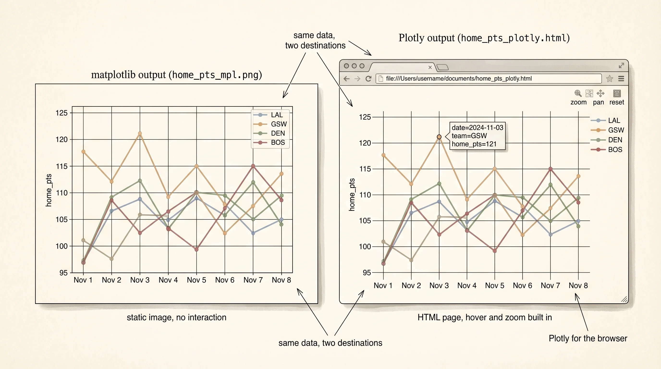
ni plots.py

Open plots.py. Start with the simplest question: how does each team's home scoring change across the four games in the slice? A line chart, one line per team, x-axis is the game date. Two versions of the same chart side by side — matplotlib first, Plotly second:

import pandas as pd
import matplotlib.pyplot as plt
import plotly.express as px
 
games = pd.read_csv("games.csv", parse_dates=["date"])
 
fig_mpl, ax = plt.subplots(figsize=(8, 5))
for team, sub in games.groupby("home_team"):
    sub_sorted = sub.sort_values("date")
    ax.plot(sub_sorted["date"], sub_sorted["home_pts"], marker="o", label=team)
ax.set_title("Home points per game (matplotlib)")
ax.set_xlabel("date")
ax.set_ylabel("home_pts")
ax.legend()
fig_mpl.savefig("home_pts_mpl.png", dpi=120, bbox_inches="tight")
print("saved home_pts_mpl.png")
 
fig_plotly = px.line(
    games.sort_values("date"),
    x="date",
    y="home_pts",
    color="home_team",
    markers=True,
    title="Home points per game (Plotly)",
)
fig_plotly.write_html("home_pts_plotly.html")
print("saved home_pts_plotly.html")

saved home_pts_mpl.png
saved home_pts_plotly.html

Two files. home_pts_mpl.png is a static image you can drop into a slide. Open it and you see four lines, a legend, and nothing else. home_pts_plotly.html is a webpage. Open it in your browser. Hover any marker and the exact date, team, and score appear in a tooltip. Click a team in the legend and that team's line disappears. Drag across a region of the chart and it zooms in. Shift-drag and it pans. Double-click to reset. You did not write any of that behavior. It came with Plotly because the library's output is real HTML rendered by Plotly.js in the browser.

The code difference matters too. matplotlib needs 5 method calls — subplots, a loop with plot, title, xlabel, ylabel, legend. Plotly Express needs 1 function call with a DataFrame and 3 column names. The shorter version is not shorter by accident; Plotly Express was designed after a decade of watching matplotlib users write the same 5 lines for every plot. It inferred the pattern and gave it a name.

A bar chart is the second-most-useful shape. Average home points per team, one bar per team, sorted tallest to shortest:

avg = games.groupby("home_team")["home_pts"].mean().sort_values(ascending=False).reset_index()
 
fig = px.bar(
    avg,
    x="home_team",
    y="home_pts",
    title="Average home points per team",
    text_auto=".1f",
)
fig.update_layout(yaxis_title="avg home_pts", xaxis_title="team")
fig.write_html("avg_pts_bar.html")
print(avg)

  home_team  home_pts
0       GSW    111.75
1       BOS    109.50
2       LAL    108.00
3       DEN    105.25

text_auto=".1f" prints the value on top of each bar to one decimal place. update_layout renames the axes. The same chart in matplotlib needs plt.bar(avg["home_team"], avg["home_pts"]) plus 4 more lines to add the text labels, because matplotlib has no first-class text_auto option. A Plotly default is often a 5-line matplotlib recipe.

A scatter plot answers a different kind of question: do two numeric columns move together? The field-goal percentage column and the home-points column should correlate — better shooting means more points — but how strongly? Plot one against the other:

fig = px.scatter(
    games,
    x="home_fg_pct",
    y="home_pts",
    color="home_team",
    hover_data=["date", "away_team"],
    trendline="ols",
    title="Field-goal % vs home points",
)
fig.write_html("fg_vs_pts.html")

trendline="ols" overlays a least-squares regression line on each team's cluster. hover_data adds extra columns to the tooltip so hovering a dot tells you the date and opponent. Open the HTML, hover the outlier in the top-right — that is the Warriors' 121-point game against Boston on November 3rd, at 51 percent from the field. The scatter plot is the first chart to reach for when you suspect a relationship. The trendline is the answer.

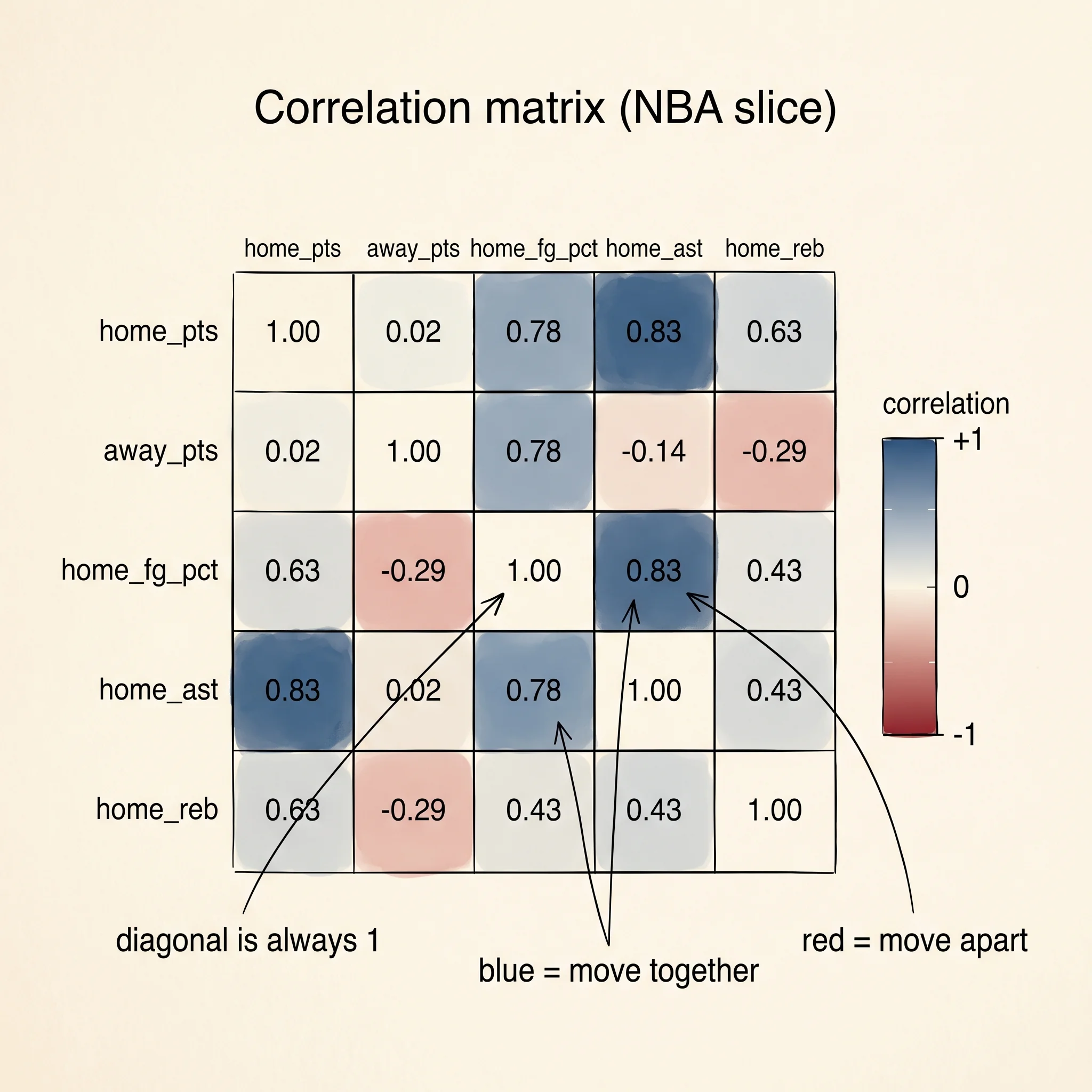
The correlation heatmap is the chart the curriculum asked for, and it is the one-minute summary of a DataFrame. Compute the correlation matrix — every numeric column against every other — and render it as a grid where color carries the number:

numeric_cols = ["home_pts", "away_pts", "home_fg_pct", "home_ast", "home_reb"]
corr = games[numeric_cols].corr()
print(corr.round(2))
 
fig = px.imshow(
    corr,
    text_auto=".2f",
    color_continuous_scale="RdBu_r",
    zmin=-1,
    zmax=1,
    title="Correlation matrix (NBA slice)",
)
fig.write_html("correlation.html")

             home_pts  away_pts  home_fg_pct  home_ast  home_reb
home_pts         1.00      0.02         0.78      0.83      0.44
away_pts         0.02      1.00        -0.29     -0.11     -0.17
home_fg_pct      0.78     -0.29         1.00      0.83      0.52
home_ast         0.83     -0.11         0.83      1.00      0.56
home_reb         0.44     -0.17         0.52      0.56      1.00

Every cell is a correlation coefficient between -1 and 1. The diagonal is always 1 because every column correlates with itself. The color scale RdBu_r draws positive correlations in blue and negative in red, with the strength scaling with saturation. The strongest off-diagonal blue is the (home_pts, home_ast) cell at 0.83, meaning teams that pass the ball more score more — unsurprising, confirmed. The (home_fg_pct, home_ast) cell is also 0.83, meaning teams that shoot better also assist more, which is a basketball cliché ("good offense comes from good passing") rendered as a number. The red cell (home_fg_pct, away_pts) at -0.29 says when your team shoots well, the other team scores slightly less — weak negative, because a better offense keeps you on offense longer.

A question worth answering from the matrix: why does home_pts barely correlate with away_pts (0.02) even though two teams playing together would share the pace of the game?

Because this slice is 16 games and pace effects are small compared to individual-team variance. A full-season DataFrame of 2,400 games would tilt this cell positive, because a fast-paced game leaves both teams with more possessions. Sample size shapes correlation. With 16 rows, anything below 0.4 in absolute value is noise.

A histogram is the fifth chart in the default kit. It bins a single numeric column and shows you its distribution — how spread out the values are, whether the middle dominates or the extremes do. Home points across all 16 games:

fig = px.histogram(
    games,
    x="home_pts",
    nbins=10,
    title="Distribution of home points (16 games)",
)
fig.update_layout(yaxis_title="games", xaxis_title="home points")
fig.write_html("hist.html")

10 bins. Most games land between 105 and 115. The tails at 98 and 121 are the outliers the scatter plot already flagged. Histograms are the fastest way to see whether a column has a clean bell curve (a normal distribution), a hard ceiling, a long right tail (a log-normal, typical of income or sports scoring), or a double hump (two hidden sub-populations). For this 16-game slice the histogram mostly tells you the sample is too small to call the shape, which is its own useful signal.

Picking between matplotlib and Plotly comes down to where the chart lives. If the final destination is paper — a LaTeX paper, a printed slide, a PNG in a PowerPoint file — matplotlib still wins, because its default typography and line weights were designed for ink. If the destination is a browser, a notebook, a dashboard, or any place a reader can hover, Plotly wins, because interactivity is free. Most data teams at modern companies lean on Plotly for internal exploration and matplotlib for published papers. You pay for both by keeping both in your venv.

You can read the past now. You have a DataFrame and charts that make it legible. What you cannot do yet is train a model that predicts anything about tomorrow's row. The next lesson reaches for the library that lets you write that model in 30 lines of Python and run it on your laptop or a GPU.